11.1. Introduction and Definitions
This chapter addresses methods, tools, and resources for developing load impact profiles—also referred to as load impact shapes or operating profiles—for the full range of DERs in the NSPM.28 This is the “Determine DER Impact on Customer Load Profiles” step in the process diagram shown in Figure 1.
Load impact profiles are needed to convey, assess, and optimize the temporal nature of DER options. In the simplest use of load impact profiles in benefits analysis, the incremental DER load impacts are multiplied by incremental avoided costs for each time interval to estimate the value of the DER impacts for use in a BCA (see Section 2.8). However, load impact profiles are applied in different ways in more complex analysis. For example, when capacity expansion modeling is used to quantify generation costs, the DER load impact profile might be used as an input to the model to develop a DER case forecast of costs (see Sections 3.2.1 and 3.2.2 for more details). In addition, the Constrained Optimization Modeling method in Section 11.2 optimizes DER impacts based on costs and other priorities so the valuation of DER impacts may occur within the model. This type of optimization includes cases where the temporal pattern of avoided costs would be used to dispatch the DER and, therefore, would be the basis of the load impact profile.
Development of DER load impact profiles generally involves analyzing two types of profiles:
- Reference Case load profile: This load profile represents what would happen in the absence of the DER(s) being evaluated in the BCA. That is, it is the expected load without the incremental effects of the DER(s) being considered. The Reference Case should include effects from all other types of DERs known to be or assumed to be present in the utility system. Therefore, the ordering of DERs is important since those being evaluated will be valued after the impacts of other DERs included in the Reference Case. The Reference Case load profile could be developed at one or more levels (end-use, whole-building, customer class, planning area, utility system, etc.).
- DER Case load profile: This is the load profile that includes the incremental impacts from the one or more DERs being evaluated.29 It could be developed to analyze an individual type of DER independently (single-DER analysis), or multiple DER types and profiles in combination (multiple-DER analysis). Analysis of multiple DER types in combination should consider resource interactions (see Section 11.2.2). Regardless of the amount of DERs assumed in the DER Case, the DERs included should ideally be optimized to meet policy objectives or grid needs (e.g., minimize utility system cost, minimize GHG emissions, minimize customer costs, avoid or defer traditional utility upgrades, improve resiliency, increase flexibility). Optimization is particularly applicable to dispatchable DERs.
The net difference between the Reference Case load profile and the DER Case load profile is referred to herein as the DER load impact profile. For some types of DERs (e.g., distributed generation), the DER load impact profile can be developed irrespective of the Reference Case and DER Case profiles. (For an example, see Section 11.4.1 which shows a simulated solar PV load impact profile that also represents the DER load impact profile.) But ultimately, the interest is in how the DERs affect the Reference Case.
Figure 44 and Figure 45 illustrate these different types of load profiles. In Figure 44, the DER under evaluation is distributed solar PV, which shows the impact of a single DER relative to the Reference Case (with no solar PV). Figure 45 provides a multi-DER example, where the Reference Case includes distributed solar PV that is already installed, and the DER Case includes estimated impacts from two other types of DERs that are being evaluated: energy efficiency and demand response, where interactions between energy efficiency and demand response have been taken into account by assuming the energy efficiency occurs before the demand response. In both examples, the net impact is a reduction in load.
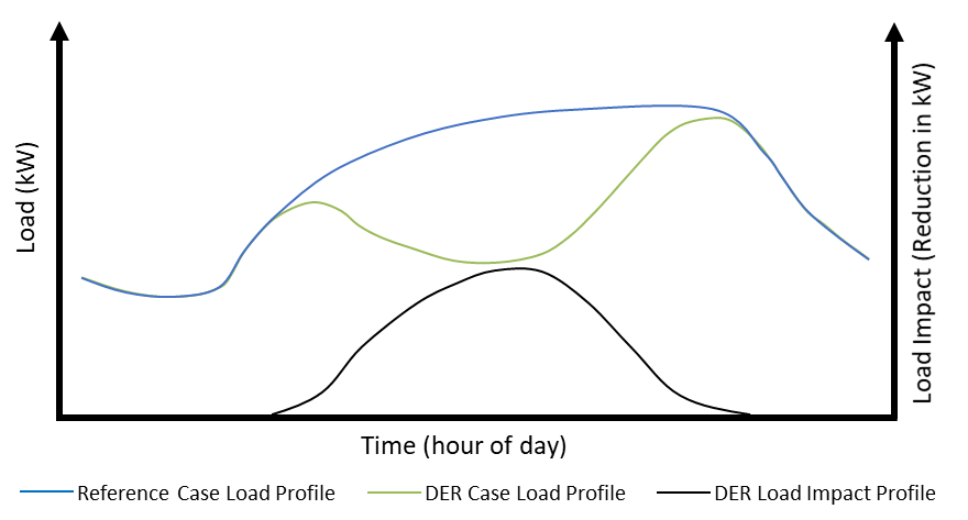 Figure 44. Illustration of load profiles: reference case, DER case, and DER load impact (DER = Solar PV)
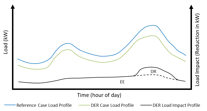 Figure 45. Illustration of load profiles: reference case, DER case, and DER load impact (DERs = EE+DR, interacted)
The remainder of this chapter is organized as follows:
- Section 11.2 describes methods for developing DER load impact profiles.
- Section 11.3 discusses applying the methods to different DER types by taking into consideration the unique load characteristics of each type of DER.
- Section 11.4 provides examples to illustrate some of the methods being used in practice.
- Section 11.5 lists examples of publicly available tools and resources to support development of DER load impact profiles.
11.2. Methods for Developing DER Load Impact Profiles
11.2.1. Overview
Developing DER load impact profiles involves the general process shown in Figure 46. To carry out the process, practitioners select from five main categories of methods: (1) simulation modeling, (2) submetering, (3) statistical approaches, (4) percent reductions, and (5) constrained optimization modeling. Within these main categories there are some subcategories with variations in approaches. In addition, several of these methods employ elements from one or more different methods. The methods described below can also be used together to form a “hybrid” approach for more complicated analysis, such as when evaluating multiple DERs in combination.

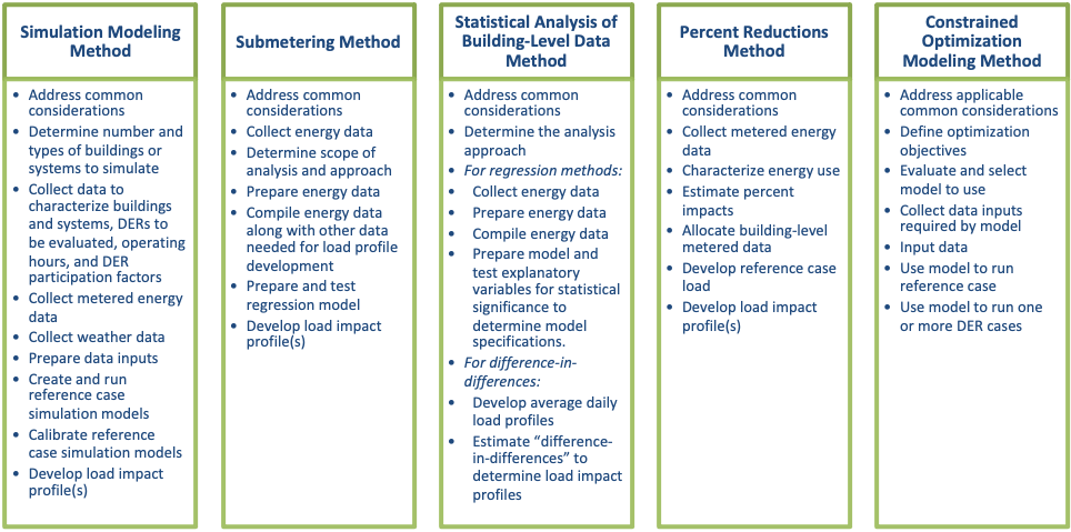 Figure 46. Overview for developing load impact profiles
Table 84 summarizes key attributes of the methods as they pertain to developing DER load impact profiles. The sections below describe the methods and attributes in more detail.
Table 84. Summary of method attributes relevant to DER load profile development
| Method |
Attribute |
| Applicability to DER Types |
Single- vs. Multiple-DER Approach |
Relative Cost |
Relative Analytic Complexity |
Relative Accuracy |
Captures Interactive Effects |
| Simulation Modeling |
All |
Multiple |
Low-Med |
Med-High |
Med |
Maybe |
| Submetering |
All |
Single |
High |
Med |
High |
No |
| Statistical Analysis of Building-Level Data |
All |
Multiple30 |
Med |
Med-High |
High |
Yes |
| Percent Reductions |
Some |
Multiple |
Low |
Low |
Low |
Maybe |
| Constrained Optimization Modeling |
Some Multiple |
Multiple |
Low-Med |
Med-High |
Med-High |
Yes |
While there have been some important advancements in application of these methods in recent years—due in part to technology advances and greater access to interval data—these basic methods for developing load profiles are not new.31 Several are regularly applied by utilities in various aspects of load research and program planning. For example, utilities use simulation modeling (often relying on a consultant or public source) for energy efficiency end-use load profiles in assessing program cost-effectiveness. Utilities also frequently use statistical regression analysis in their load research to derive sample-weighted hourly load profiles for different rate classes in a cost of service study, and statistical regression analysis with class load research data is sometimes used for market settlement as well. Additionally, many utilities use statistically adjusted end-use forecasts as the basis for their load forecasts in IRPs. These methods are also commonly applied in program impact evaluation (EM&V). Load profiles derived as part of a past or current impact evaluation for a DER program or pilot are directly relevant to a BCA since those impacts help inform load forecasts and utility planning with respect to DERs.
11.2.2. Common Considerations
Despite inherent differences in the methods, there are several common considerations in developing DER load impact profiles. At the most basic level, a solid understanding of the types and characteristics of the DERs to be evaluated and the specific objectives of the BCA is essential. Another fundamental consideration is accounting for resource interactions when conducting multiple-DER analysis. In addition, timescales and metrics for the avoided costs and DER load impacts should ideally match. Any analysis should also address and quantify uncertainty to the extent practicable. These basic considerations are described more fully below:
- DERs to be evaluated: The types of DERs to be evaluated, customer classes of interest, and the objectives of the BCA are essential considerations in planning for and developing DER load impact profiles.
- Resource interactions: Interactions between different resources must be accounted for to estimate impacts accurately. Some methods can capture and isolate interactions better than others. Conceptually, accounting for resource interactions means that the Reference Case load profile is adjusted after each DER is analyzed. That way, as subsequent DERs are added to the analysis, their impacts will be calculated relative to the adjusted baseline. Factors to consider include “loading order” of the resources (defined as the order the DERs are added to the analysis, i.e., what happens first) and how the DERs are expected to interact (will they compete, complement each other, or have no effect on one another?). For example, see LBNL 2020 EE-DR for a conceptual framework to describe energy efficiency and demand response interactions.
- Time interval: Hourly intervals are generally the preferred choice when developing load profiles if the incremental cost information is available or can be estimated at that granularity. For some DER use cases, sub-hour intervals may be desirable if there are load impacts that are not evident in hourly intervals. In others, it might be sufficient to estimate average load impacts for key sub-annual periods, such as winter and summer or on- and off-peak periods.
- Time stamp convention: When working with multiple datasets containing interval data, it is important to make sure the data align. Considerations include whether the time stamp reflects the beginning or end of the interval and how daylight savings time is handled.
- Time period: The key time periods that reflect DER operation should be captured in the load profiles. The time periods may be specific hours, days, weeks, months, seasons, or years. Day-types—such as average weekday, average weekend day, monthly peak day, winter system peak day, and summer system peak day—are often used to represent time periods of interest.
- Study period: The BCA study period should be long enough to include the full operating life of the DER being analyzed. Therefore, DER load impact profiles and corresponding incremental costs ideally should be developed to represent each year during the life of the DERs being evaluated to capture any expected variations in load impacts and incremental costs across years. Variations in load impacts may be due to persistence factors (i.e., degradation of impacts over time) or increases in adoption of DERs. In multiple-DER analysis, combined impacts in later years may change due to different lifetimes for different types of DERs.
- Load metric: The load metric (kW, kWh, therm, etc.) must align with the avoided cost metric ($/kW, $/kWh, $/therm, etc.). With sub-hour interval data, it is also important to pay special attention when calculating kWh (an energy unit) based on kW (a power unit). For example, to convert 15-min kW data to 15-min kWh, multiply each kW measurement by ¼ hour. To convert 15-min kW data to hourly kWh, average the four 15-min kW measurements for each hour. To convert 15-min kWh data to hourly kWh, sum the four 15-min kWh values within each hour.
- Uncertainty: All estimation methods have uncertainty. Some types of errors are easier to quantify than others. Best practice is to identify and quantify (when possible) sources of errors and then report them by creating confidence intervals around point estimates.
Option 1: Simulation Modeling Method
Energy simulation modeling uses physics-based principles to estimate DER load impact profiles. Building energy simulation models use available primary or secondary data on building characteristics to simulate how buildings and sub-systems use energy. Very detailed models can be built up to represent specific buildings or, alternatively, building prototypes can be developed or obtained from open sources to represent different customer classes of interest. They can also be used to optimize building characteristics and DER measures (like energy efficiency, demand response, and electrification) to minimize costs. Other types of simulation models focus on estimating (and optimizing) impacts from distributed generation and distributed storage systems. Calibrated simulation models reconcile results from the physics-based models to actual metered energy data.
The simulation modeling method involves the key steps shown in Table 85.
Table 85. Steps to develop DER load profiles using simulation modeling
| Step 1 |
Address the common considerations listed above
|
| Step 2 |
Determine the number and types of buildings or systems to simulate
If a sample of buildings will be analyzed to represent a larger population, determine the size of the population. |
| Step 3 |
Collect data to characterize the buildings and systems, DERs to be evaluated, operating hours, and DER participation factors
Data to describe buildings and operation could come from actual sites, utility surveys that generalize characteristics by customer type (e.g., data collected during a baseline study), secondary sources, or a combination of sources. The data requirements will vary depending on the type of building, type of model, and level of customization required. |
| Step 4 |
When available, collect metered energy data (and energy cost information if doing financial analysis along with load impacts)
The energy data could be in the form of monthly billing data, smart meter data, and/or submeter data from specific end-uses or DERs being evaluated. The type of energy data to use will depend on what is available. Usually, when choosing the simulation modeling approach to estimate building energy use, only whole-building energy data is available, and it may only be available at the monthly level; but it is possible to have more granular data, including from submeters. Another determining factor for the type of energy data to collect is whether the model is predicting impacts due to various DER scenarios or whether the model is estimating impacts after DER implementation. If the former, the collected energy data would be for the Reference Case period. If the latter, the collected energy data would be for the DER Case period as well as the Reference Case period, if available. |
| Step 5 |
Collect weather data
The weather data should correspond with the timescales of the study. Simulations are often conducted at the hourly level to represent annual operation (“8760” models). The weather should also reflect the conditions of interest for the study (actual weather, normal weather, something else). |
| Step 6 |
Prepare the data inputs
Conduct basic cleaning and validation of the energy data. Organize all data inputs to align with the appropriate simulations. |
| Step 7 |
Create and run the Reference Case simulation models
Develop a Reference Case model for each building or system type. This could include developing a prototype or using or adapting a prototype or model from a secondary source. The output will include simulated energy loads at the building and subsystem level in hourly (or possibly sub-hourly) increments. |
| Step 8 |
Calibrate the Reference Case simulation models
If available, use metered energy data from the Reference Case period to calibrate the model.32 Examples of when appropriate Reference Case metered energy data may not be available include new construction, building expansions, changes in industrial processes, other non-routine events, or if consumption and sales are different because of onsite generation (this would be a problem if the model is designed to capture consumption and the metered energy data represents sales). |
| Step 9 |
Use the calibrated model to simulate DER Cases
Run one or more DER Case simulations for each building or system type. This involves adapting the Reference Case model to reflect the DERs to be assessed. The DER Case should include all DERs under evaluation for the given scenario. |
| Step 10 |
Calibrate the DER Case simulation models (if DERs are already implemented)
Use metered energy data from the DER period to calibrate the models for buildings that have already implemented DERs. |
| Step 11 |
Develop load impact profile(s)
Calculate the DER load impact profile by subtracting the loads for the DER Case from the Reference Case for each interval and calculate for each building or system type and aggregate and expand to the populations of interest. |
The following attributes characterize the simulation modeling method:
Applicability to DER Types: The simulation modeling method applies to all DER types.
Single- vs. multiple-DER approach: The simulation modeling approach can be used for single or multiple DERs, depending on the package of DERs being evaluated. For example, a distributed generation system would probably be modeled separately from energy efficiency measures, while a package of energy efficiency and electrification measures could be evaluated together in the same simulation model. There is a distinction because building energy simulation models developed with engines like EnergyPlus and DOE-2 simulate buildings and their systems and can be used to estimate the effects of various actions—including energy efficiency measures, electrification, and demand response strategies—on end-use systems, while other models like PVWatts simulate distributed generation systems for a given building or topography.
Cost and complexity: This method has a low-to-medium cost and medium-to-high complexity compared to other methods. Factors that influence the cost and complexity are the sophistication requirements for the models (how closely does the model need to match an actual building vs. a “typical” or average building), the sample size (how many buildings or systems need to be simulated), and the DERs to be evaluated (how many and what type of DER scenarios are needed). The lowest cost and simplest application of this measure is the use of free software with user-friendly interfaces to evaluate a small number of sites and for a limited set of DER scenarios. An example of this would be using PVWatts to estimate performance of solar PV (see Section 11.4.1). The highest cost and most complex application of this method is to create a large number of detailed building energy models using a building simulation engine such as EnergyPlus or DOE-2; that would require considerable expertise and time. Generally, creating a building energy model from scratch would not be required because there are several software interfaces available (including OpenStudio, eQUEST, and BEopt) to simplify use of simulations engines. In addition, developing prototypes to represent the average building for each customer class and building type of interest is easier than developing unique simulation models for each specific building. It is also possible to use prototypes from secondary sources, as long as there is the capability for customization where needed. See Section 11.5.2.a for descriptions of some publicly available building simulation models and tools.
Accuracy: In general, this method has medium accuracy compared to other methods. Models that calibrate to metered data are more accurate than those that do not. The accuracy also depends on the quality of the inputs used to characterize the buildings. There are often challenges collecting sufficiently detailed data on building characteristics to create an accurate model or prototype. One advantage of this method is that individual DER impacts can be readily isolated from building-level impacts. One disadvantage is that the models do not capture behavioral effects.
Interactive effects: The ability of simulation modeling to account for interactive effects depends on the model. Some building energy simulation models are able to account for interactive effects between some types of DERs. This attribute is very useful when looking at different combinations of DERs as well when assessing the effects of a DER on other end-uses, such as how building envelope measures affect the HVAC load. (See LBNL 2020 EE Buildings for an example of using simulation models to analyze interactions between energy efficiency and demand response on regional grid scales.)
Option 2: Submetering Method
Submetering uses measurements of energy or proxies of energy (current, voltage, power factor) to develop load profiles. In the simplest application of this method, the measurements are used directly without additional manipulation or adjustment. However, statistical approaches are often used to analyze the data and to correlate impacts to explanatory variables.
The submetering method involves the key steps described in Table 86.
Table 86. Steps to develop DER load profiles using the submetering method
| Step 1 |
Address the common considerations listed above
|
| Step 2 |
Collect the energy data
Key considerations include:
- Data source: Submeters, building automation systems, data loggers, etc.
- Data type: Energy consumption, distributed generation output, distributed storage, or electric vehicle charging/discharging measurements, other
- Data scale: Sample size, population of customers (or systems) included in aggregate analysis
- Data availability: Is submeter data available to represent both the Reference Case and DER Case, or just one or the other?
|
| Step 3 |
Determine the scope of the analysis and approach
Key considerations include:
- Type of load profile(s) to be developed: This will depend on the available submeter data and type of DER. For energy efficiency and demand response, if only Reference Case data is available (or only DER Case data is available), then an end-use load profile can be developed but the load impacts will need to be estimated with other methods, such as simulation modeling or percent reductions. However, if the submeter data reflects both Reference Case and DER Case loads, the DER load impact profile can be estimated as the difference of the two. For other DERs like solar PV, battery storage, electric vehicles, and electrification, the DER load impact profile can be developed directly since the submeter would be recording actual operation of the DER instead of a change in operation of a given end-use.
- Analysis approach: In some cases, submeter data might be used directly without further manipulation to convey the load profiles for the measurement period. However, it is far more common to use statistical regression analysis to develop and analyze load profiles from sub-metered data; generally linear regressions are employed. Statistical regressions help quantify relationships between the load and one or more explanatory variables. If the right submeter data is available, regression models can include both Reference Case and DER Case variables so that DER impacts can be calculated from the model. These types of models allow users to estimate impacts under different conditions by varying values for the explanatory variables.
|
| Step 4 |
Prepare the energy data
Conduct basic data cleaning and validation procedures and aggregate data to data intervals of interest. For example, if submeters record data at intervals of 5 mins and hourly profiles are desired, aggregate the data to hourly levels.
If the data is not going to be regressed, prepare a dataset for conveying load profiles for the time period and data interval of interest. If applicable, calculate load impacts by aligning Reference Case and DER Case data (by time of day, day of week, etc.) and computing the difference.
If using regressions, complete Steps 5-7. |
| Step 5 |
Compile the energy data along with other data needed for load profile development
This includes data such as weather data, calendar data, customer data, other variables. |
| Step 6 |
Prepare and test the regression model
This involves testing explanatory variables for statistical significance and determining the best model specification. |
| Step 7 |
Develop load impact profile(s)
Apply the model to estimate the Reference Case, DER Case, and/or DER load impact profiles, as applicable. Typically impacts are estimated at an average customer level for a given customer class and then reconciled to the population of interest. The impacts should capture the study period and conditions relevant for the BCA (e.g., time, day, season, weather). The choice of weather applied in the model—actual weather, normal weather, event day weather, or something else—should be consistent with the type of DER being analyzed and should correspond to incremental cost data. |
The following attributes characterize the submetering method:
Applicability to DER Types: The submetering method potentially applies to all DER types but is not the best choice for behavioral-based or strategy-based DER analysis. For example, submetering a solar PV system alone cannot discern whether or not the customer consumed more energy after installing solar PV as a result of now having lower energy bills; in other words, it cannot capture rebound effects. Additionally, though submetering can readily capture how a customer charged their electric vehicle under a particular rate, a more rigorous experimental study design leveraging submetering would be required to assess how different rates would yield different charging profiles.
Single- vs. multiple-DER approach: Submetering is inherently a single-DER analysis approach, however, it can be used for multiple-DER analysis if all DERs and end-uses known to be affected by DERs are sub-metered.
Cost and complexity: This method has a high cost and medium complexity compared to other methods. The simplest and least-cost application of the method is for DER impacts that can be measured directly, such as for solar PV systems, batteries, electric vehicles, and electrification. It is also applicable to energy efficiency and demand response measures; but the expense, complexity and, in some cases, the time commitment is greater since loads should ideally be measured for the Reference Case and DER Case to calculate the load impact profile.
Accuracy: The accuracy of submetering is high relative to other methods since it involves direct temporal load measurements of DERs or end-uses known to be affected by DERs.
Interactive effects: Submetering cannot account for interactive or fuel-switching effects unless all other systems expected to be affected by the DER are also sub-metered.
Option 3: Statistical Analysis of Building-Level Data Method
This method uses statistical approaches to model Reference Case and DER Case loads and determine load impacts from building-level interval energy data. Typically, the data is from utility smart meters that record load data in sub-hourly or hourly intervals.
Statistical analysis of building-level data involves the key steps in Table 87.
Table 87. Steps to develop DER load profiles using statistical analysis of building-level data
| Step 1 |
Address the common considerations listed above
|
| Step 2 |
Determine the analysis approach
Examples of statistical approaches for analyzing building-level interval data include difference-in-differences, fixed effects regression, and customer-specific regression: 33, 34, 35
- Difference-in-differences: This method is applied when comparing a control group to a treatment group. The control group’s energy use serves as the Reference Case, while the treatment group’s energy use informs the DER Case. Customers in the treatment group have been participants in a DER program. In this method, interval data is collected during the pre-treatment period and treatment period for both the control group and the treatment group.
- Fixed effects regression: As noted earlier, regression models help quantify relationships between the load and one or more explanatory variables like weather, customer type, and time-related variables. Fixed effects regressions can be used to analyze a Reference Case and a DER Case for a group of customers that have participated in a DER program, or to compare a control group with a treatment group. In either application, interval data is collected during the pre-treatment period and treatment period for all customers in the sample.
- Customer specific regression: This method is useful when analyzing impacts for customers that have very different load profiles from one another. The regression models are developed for each customer participating in the program and then the results are aggregated into customer groups of interest. For example, this method works well for estimating load impact profiles for commercial and industrial customers participating in aggregator-managed demand response programs. In that application, the DER Case is an event day and the Reference Case is a non-event day.
|
| For the regression methods, the remaining steps (Steps 3a-7a) are essentially the same as Steps 3-7 in the Submetering method. |
| Step 3a |
Collect the energy data
|
| Step 4a |
Prepare the energy data
|
| Step 5a |
Compile the energy data
|
| Step 6a |
Prepare the model and test explanatory variables for statistical significance to determine the best model specifications
|
| Step 7a |
Develop load and load impact profiles from the models for the conditions of interest
|
| For difference-in-differences, the remaining steps are as follows:36 |
| Step 3b |
Develop average daily load profiles
Develop profiles for each customer in the control group and treatment group, for each day type of interest and for both the pre-treatment period and the treatment period. For the customer segments of interest, average the daily load profiles across the customers to get average per-customer load profiles for each segment. The result will be average Reference Case (control group) load profiles and average DER Case (treatment group) load profiles for each customer segment and day type.
|
| Step 4b |
Estimate the “difference-in-differences” to determine the load impact profiles
- Estimate the first difference. For each customer segment and each day type, calculate the difference between the control group’s average load and the participant group’s average load. Calculate for both the pre-treatment and treatment periods.
- Estimate the second difference. Subtract the first difference for the pre-treatment period from the first difference for the treatment period to get an estimate of the load impacts that corrects for pre-treatment differences between the control group and treatment group. Calculate for each customer segment and day type of interest. Aggregate the impacts to the population
|
A variation to the methods described above is Normalized Metered Energy Consumption (NMEC). The NMEC approach is emerging as part of the next generation measurement and verification concept (“Advanced M&V” or “M&V 2.0”). This approach entails using building-level (or subsystem level) interval data along with automated modeling processes—often employing statistical regressions—to assess overall load impacts for the building (or subsystem). The key differentiator from the other regression approaches already discussed is the analysis is done in “real time” to provide fast feedback on the performance of DERs. This fast feedback helps building operators understand and manage energy use more dynamically and allows for more accurate and timely estimates for pay-for-performance programs. Advanced M&V leveraging the NMEC approach also shows potential as an enabling method for assessing the performance of grid-interactive efficient buildings at the fine timescales and high speeds required for grid services. These same qualities of fine timescales and high speed are well suited for assessing temporal impacts at the building or subsystem level from non-wires solutions. However, advanced M&V and its application to grid-interactive efficient buildings and non-wires solutions is still in the early stages.37
The following attributes characterize the statistical analysis of building-level data method:
Applicability to DER Types: The statistical analysis of building-level data method applies to all DER types.
Single- vs. multiple-DER approach: This is a multiple-DER analysis approach since impacts are calculated at the building level. However, it is difficult to attribute impacts to individual DERs without more complex models or submetering.
Cost and complexity: This general method category has a medium-to-high cost and high complexity compared to other methods. Of the statistical approaches, the simplest and least cost is the difference-in-differences method. It is the easiest to apply since it is based on direct comparisons of loads for the
Reference Case and DER Case. Fixed effects regression is more complex (and therefore more costly) than difference-in-differences because of the need to develop a regression model, but it is less complex and less costly than customer-specific regressions since the latter requires developing and testing models applicable to multiple customer types. The NMEC method is the most complex and costly since it involves very sophisticated models and may require paying for a software service.
Accuracy: The accuracy of this method is relatively high (at least at the building level) since the loads are based on actual interval meter data for both the Reference Case and the DER Case. This method has the advantage over other methods in that it captures behavioral effects.
Interactive effects: Whole-building statistical approaches inherently capture interactive effects of measures for a given energy source (usually electricity). However, they cannot account for fuel-switching effects unless the other affected fuels are also analyzed.
Option 4: Percent Reductions Method
This method applies estimates of percent reductions in DER load impacts (e.g., energy savings or peak demand reductions) to Reference Case load profiles to develop DER load impact profiles. The Reference Case load profiles may be obtained from public sources or developed with one of the other methods described above.
The percent reductions method involves the key steps in Table 88.
Table 88. Steps to develop DER load profiles using the percent reductions method
| Step 1 |
Address the common considerations listed above
|
| Step 2 |
Collect metered energy data
This includes annual and monthly utility data, and any hourly or sub-hourly interval data that is available at the whole-building or submeter level for customers included in the analysis scope. |
| Step 3 |
Characterize energy use
Use primary or secondary sources to characterize the buildings and subsystems (including end-uses and technologies) for each customer class and building type of interest. Data could come from actual sites, utility surveys that generalize characteristics by customer type (e.g., data collected during a baseline study), secondary sources (e.g., U.S. EIA), or a combination of sources. Identify any customers with onsite generation, such as those with solar PV who participate in net-metering programs. |
| Step 4 |
Estimate percent impacts
Use engineering calculations, models, measurements, or secondary sources to estimate the percent impacts from the DERs for the time periods relevant to the use case. For example, specific day types and specific hours of the day may be relevant for a demand response use case, while it may be sufficient to estimate impacts at the seasonal or annual level for an energy efficiency use case. In some use cases the percent impact may represent an overall building-level impact (e.g., for a behavioral program), but often the percent impact would be calculated at the end-use level (e.g., installing efficient lighting or HVAC equipment). |
| Step 5 |
Allocate building-level metered data
This will result in an estimate of average per-customer energy use for each customer class and building type. It involves the following sub-steps:
- Compile metered data for all customers within a given customer class and building type.
- Calculate the average annual (or more granular) energy use per customer (or sq ft) for each customer class and building type.
- When conducting end-use level analysis, allocate the average energy use to end-uses and technologies using the customer characterization data.
|
| Step 6 |
Develop Reference Case load
This step is carried out for all customer classes and building types and involves two sub-steps:
- Using load profiles obtained from primary or secondary sources (see Section 11.5.1), compile a set of unitized load profiles, preferably at the end-use and technology level, to represent each customer class and building type of interest. In a unitized load profile, the sum of the values for the period (usually increments of 8760 hours per year) equals 1.0. Therefore, the value for each increment is a small fraction. These fractional values can be multiplied by a total load for the period (usually an annual load) to develop a load profile.
- Multiply the unitized load profiles by the average customer energy use at the building level (or at the end-use and technology level). The calculation will involve multiplying each fraction in the unitized load profile by the energy use value for the period (e.g., annual kWh/customer or annual kWh/sq ft).
|
| Step 7 |
Develop load impact profile(s)
Apply the estimated percent impacts to the Reference Case load profiles. There are a few ways to do this depending on the use case:
- For building-level estimation, apply percent impacts to the building-level Reference Case profile to develop a load impact profile. This method assumes that the impact profile will have the same shape as the Reference Case profile, but with a lower magnitude.
- For end-use or technology level estimation, apply percent impacts to the corresponding end-use or technology level Reference Case profile to develop separate load impact profiles for each end-use or technology. These can then be stacked to determine the combined impact at the building level.
- When conducting this analysis for specific intervals—such as to assess the impact of demand response during the system peak hours—the percent impacts would only be applied to those intervals.
|
The following attributes characterize the percent reductions method:
Applicability to DER Types: The percent reductions method is most appropriate for energy efficiency and certain types of demand response (specifically load shed) when the timing of the load impacts is known or can be readily estimated from Reference Case load profiles.
Single- vs. multiple-DER approach: This is a multiple-DER approach. Separate percent reductions for individual DERs are estimated separately. Then, they are stacked to create a combined load impact profile. When stacking the DER impacts, it is important to account for resource interactions; this involves adjusting the Reference Case load between each additional DER so that the overall impacts are not overstated. (See Section 11.4.2 for an example of using percent reductions for multiple-DER analysis.)
Accounting for Resource Interactions: As a simple example, consider a Reference Case load of 100 kW that is reduced by 10% to 90 kW by the first DER, resulting in a 10 kW impact. The second DER has a percent reduction of 5%. If applied to the original load of 100 kW, the load impact of the second DER would be 5 kW; however, it would be 4.5 kW if applied to the adjusted 90 kW reference load. If resource interactions were not accounted for, the impact would be 10 kW + 5 kW = 15 kW, which is overstated. To account for resource interactions, the appropriate stacked impact should be 10 kW + 4.5 kW = 14.5 kW.
Cost and complexity: This method has a low cost and low complexity relative to the other methods.
Accuracy: The accuracy is relatively low since temporal load impacts are not measured or simulated; instead, the method’s underlying assumption is that the DER load impact profile has the same general shape as the Reference Case profile during the time period under evaluation, but loads are adjusted upwards or downwards. Nevertheless, this method works very well as a planning tool for energy efficiency and demand response resources.
Interactive effects: It is possible to account for interactive effects using the percent reductions method if the interactive effects are known and can be estimated. For example, efficient lighting measures affect HVAC loads. So, to account for the interactive effects, both the percent reduction in the lighting load and the percent changes (increase or decrease) in the HVAC loads would need to be calculated.
Option 5: Constrained Optimization Modeling Method
Constrained optimization modeling is a special class of simulation models designed to make it easier to compare and optimize different DER scenarios for a given site (or other topography) to meet specific objectives (minimizing costs, maximizing resiliency, minimizing greenhouse gas emissions, etc.). This type of modeling is particularly useful for DERs that can be more flexible and responsive to fluctuating grid needs, such as distributed storage.
There are several tools available to the public for evaluating DER options; some are free, and some are not. Section 11.5.2.b summarizes a few constrained optimization modeling tools, including Homer Energy’s HOMER Grid and HOMER Pro, NREL’s System Advisory Model (SAM) and REopt Lite, LBNL’s DER-CAM, and Sandia National Laboratories’ QuESt. (See Nguyen 2021 for a comparison of these and other models.) The sophistication and capabilities vary across the models. A common feature is that each model requires user input of parameters such as location, energy costs, energy loads, and information to describe the site and DERs of interest. Some models are equipped with libraries of load profiles to select from when setting up the model and will also pull in other data (solar, wind, weather data) from secondary sources. In addition, some models output very granular time series data on how the DERs serve the building loads, including hourly performance profiles. Others report optimized cost and performance metrics that can be used along with load profiles from within the model or from other sources to estimate DER load impact profiles.
Table 89 shows the basics steps for using an existing modeling tool to optimize DER alternatives.
Table 89. Steps for optimizing DER alternatives using an existing modeling tool
| Step 1 |
Address the applicable common considerations listed above
|
| Step 2 |
Define optimization objectives
Variable(s) to be minimized or maximized and the constraints. |
| Step 3 |
Evaluate and select a model to use
See Section 11.5.2.b for a few options. |
| Step 4 |
Collect data inputs required by the model
These will likely include information to define the site, loads, location, weather, energy prices, existing DERs, and DERs to be evaluated. |
| Step 5 |
Input data
Models may have a combination of custom inputs and drop-down menus or libraries from which to select. |
| Step 6 |
Use the model to run Reference Case
The output will reflect the loads and costs without the DERs to be evaluated. |
| Step 7 |
Use the model to run one or more DER cases
For each DER Case, the output will reflect the loads and costs for an optimized scenario. |
The following attributes characterize the constrained optimization modeling method:
Applicability to DER Types: These types of models are designed to optimize a range of DER options to meet different objectives. However, in the context of evaluating DERs for a BCA, constrained optimization modeling is most applicable to dispatchable DERs that can provide grid services, i.e., distributed storage, electric vehicles (vehicle-to-grid), distributed generation plus storage and/or electric vehicles, and use of these technologies for demand response.
Single- vs. multiple-DER approach: This is primarily a multiple-DER analysis approach since different combinations of DERs can be simulated and optimized. (See Section 11.4.3 for an example of constrained optimization modeling of solar PV and storage.)
Cost and complexity: The cost of this method is low-to-medium, and the complexity is medium-to-high relative to the other methods. The cost will depend on whether the model is free or requires a license. The complexity will depend on how much and what type of data is required, how many sites and scenarios will be modeled, and the model’s user interface.
Accuracy: The accuracy of the model and model output are a function of the sophistication of the model, the underlying algorithms and assumptions used in the model design, and the quality of the inputs. Relative to the other methods, the accuracy would be in the medium-to-high range if the inputs represent the use case reasonably well.
Interactive effects: This method accounts for interactive effects when the models are used to optimize combinations of DERs.
11.2.3. Load Profile Considerations for Fossil Fuels
Some types of DERs reduce fossil fuels consumed by the customer. Examples include energy efficiency through natural gas measures, interactive effects from electric energy efficiency measures, and electrification (fuel switching). Electrification may be for building end-uses such as heat pumps for HVAC or water heating, for transportation (electric vehicles), and even for distributed generation and storage such as solar PV and batteries displacing fossil fuel generators. The fossil fuels may be in the form of natural gas, propane, oil, gasoline, or diesel.
A BCA analysis will only require load profiles for fossil fuels to the extent that incremental cost information is available at the temporal level. Temporal data for fossil fuel loads and costs are generally less available and often less granular than temporal data for electric loads and costs. When data is available, the load impacts should ideally be analyzed with the same time interval as the incremental fuel cost data. Load profiles for affected fossil fuels should be developed to correspond to the time periods they would have been operating in the absence of the given DERs. This may or may not correspond to the DER load impact profiles.
Many of the methods described in this chapter apply to fossil fuel analysis—when and if there is an important temporal relationship with incremental cost. Applicability of the methods is particularly true for fuels, like natural gas, that are supplied to buildings and metered, or for fossil fuel-fired equipment that can be sub-metered. In those cases, simulation modeling, submetering, statistical approaches, and percent reductions are all good options. Granular load profile analysis for fuels used in transportation is not likely to be applicable in a BCA.
11.3. Applying Methods to Different Types of DERs
There are various factors to consider when applying methods to develop load impact profiles for different types of DERs. Specifically, some methods are more applicable to certain DERs than others. In addition, each type of DER has a unique set of characteristics that must be taken into account when developing load impact profiles. This section explains these factors.
11.3.1. Mapping of Methods to DER Types
The method attributes discussion in Section 11.2 described the general applicability of each method to specific types of DERs. Table 90 summarizes this mapping of methods to DER Types. Presence of a check mark indicates the method is applicable to the given DER type.
Table 90. Mapping of methods for developing load profiles to DER types
| Method |
DER Type |
| Energy Efficiency |
Electrification |
Distributed Generation |
Distributed Storage |
Electric Vehicles |
Demand Response |
| Simulation Modeling |
|
|
|
|
|
|
| Submetering |
|
|
|
|
|
|
| Statistical Analysis of Building-Level Data |
|
|
|
|
|
|
| Percent Reductions |
|
|
|
|
|
|
| Constrained Optimization Modeling |
|
|
|
|
|
|
Note: Constrained optimization modeling of distributed generation applies especially in the context of distributed generation plus distributed storage and/or electric vehicles.
In some ways, specific characteristics of the DERs and their load profiles make a given method appropriate. For example, the percent reductions method is really only applicable to traditional energy efficiency and certain types of demand response (e.g., load shed) because those types of DERs yield load reductions during predictable hours of the day. The relevant hours correspond to when the end-use equipment operates (energy efficiency) or during known peak periods (demand response). In contrast, constrained optimization models apply for DERs that can be more flexible, like distributed storage and electric vehicles, as well as for when demand response is used as a more flexible resource (i.e., through use of grid-integrated end-use equipment and controls). The following subsections discuss characteristics associated with DERs and their load profiles in more detail.
11.3.2. Key Characteristics of Load Profiles by DER Type
Different types of DERs have different effects on Reference Case load profiles. Whether those effects increase or decrease loads, are persistent or temporary, are controllable or not, and are more evenly or less evenly distributed across the profile depend on the type of DER. Figure 47 below presents a set of graphics showing examples of how the different types of DERs can affect load profiles. The graphs compare Reference Case and DER Case profiles for hypothetical commercial and residential buildings. These are simplified examples. Actual load profiles will depend on the specific use cases and could look very different than these.
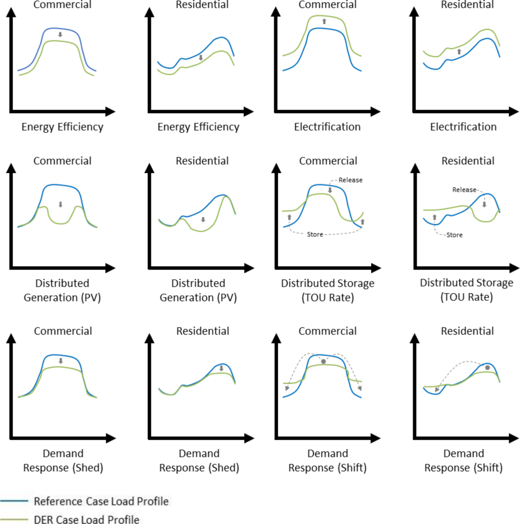 Figure 47. Illustrative load profiles for DERs in commercial and residential buildings
The subsections below describe characteristics of load and load impact profiles for three groupings of DERs: (1) more passive resources (energy efficiency and electrification); (2) more active resources (distributed storage, electric vehicles, and demand response); and then (3) distributed generation, which could be active or passive depending on the use case. The descriptions include a discussion of key factors to consider when developing load impact profiles.
11.3.3. Energy Efficiency and Electrification
Traditional energy efficiency and electrification measures can be thought of as passive resources that either decrease (energy efficiency) or increase (electrification) loads relative to a reference case. The timing of those reductions or increases in loads correspond to when the affected end-uses consume energy. For example, efficient lighting will yield a greater reduction in residential loads during the evening, efficient air conditioning will yield greater reductions during summer afternoons and switching from a gas furnace to a heat pump increases loads more during winter nights. Thus, there are important temporal aspects to these load changes, but they tend to be well correlated with weather, seasons, daylight, and building operation. The benefit of this passive attribute is that the load impacts are more reliable, and their timing is more predictable. In addition, once the load impact profiles are well characterized for one jurisdiction, they are more readily adaptable to another that has a similar climate and market, which greatly simplifies development of load impact profiles for a BCA. From a grid services perspective, a downside of this passive attribute is there is less flexibility to alter the load profiles to meet grid objectives.
A new class of resources is emerging that is more active and therefore more dispatchable. A few examples include smart thermostats, smart appliances, grid-integrated water heaters, and electric vehicles. These resources can be thought of as energy efficiency measures—or electrification for the case of electric vehicles—but their controllability features allow them to be used for other grid services, such as for addressing localized or system-wide capacity constraints. Therefore, they integrate features of energy efficiency and demand response and are sometimes referred to as integrated DSM (iDSM) resources. Load impact profiles for iDSM will vary based on things like how much flexibility they offer, how they are controlled, and when they are needed by the grid, which means that developing load impact profiles requires consideration of different use cases.
The subsections below list some specific aspects to consider when developing load impact profiles for traditional energy efficiency and electrification resources.
11.3.3.a. Energy Efficiency
Key considerations for developing load impact profiles for energy efficiency resources include approaches for:
- Determining savings (i.e., engineering algorithms, benchmarking studies, direct measurements, or whole-building statistical approaches),
- Disaggregating building-level loads to end-use level when using whole-building approaches, and
- Spreading impacts across a representative load profile when only monthly or annual savings have been determined. A common assumption for energy efficiency is that the load impact profile has the same shape as the load profile but depending on the measure or portfolio of measures this may or may not be the case.
The first four methods in Section 11.2 apply to energy efficiency resources: simulation modeling, submetering, statistical analysis of building-level data, and percent reductions.
11.3.3.b. Electrification
Key considerations for developing load impact profiles for electrification include:
- Determining how the electric technologies change the end-use load shapes (e.g., for HVAC and water heating). Unlike for energy efficiency measures, electrification always creates a new or very different load profile than the Reference Case of a fossil fuel-fired end-use. Therefore, the load impact profile will have a different shape than the Reference Case.
- Differentiating between unmanaged and managed electrification loads. For example, load impact profiles from unmanaged electric storage water heaters and electric vehicles should be analyzed differently than managed electric storage water heaters and electric vehicles. (See Section 11.3.4 for a discussion of managed loads.)
- Understanding fuel-switching implications and when it will be necessary to develop a fossil fuel load profile (see Section 11.2.3 for more information).
The first three methods in Section 11.2 apply to electrification resources: simulation modeling, submetering, and statistical analysis of building-level data.
11.3.4. Distributed Storage, Electric Vehicles, and Demand Response
The attribute that distributed storage, electric vehicles, and demand response all have in common is they are (or have the potential to be) active resources. They can be managed by the customer or directly by the utility to respond to a price signal or to a reliability or resiliency event. Their load impact profiles will vary depending on the use case. General considerations related to developing load impact profiles include the following:
- The reliability and accuracy of the estimated load impact profile depend on if and how the resource(s) is controlled. For example, direct control leads to greater reliability and less uncertainty than a time-of-use rate, which is designed to influence customer behavior.
- Optimizing how and when the resource is used to meet priorities. This is where the constrained optimization method comes in, to evaluate various scenarios and their load impact profiles.
- Whether bulk power or distribution system values are needed. Distribution system analysis is more complicated and less accurate.
In addition to the general considerations, the subsections below list some specific aspects to consider when developing load impact profiles for each of these three types of resources.
11.3.4.a. Distributed Storage
For distributed storage, key considerations include:
- The type of storage (electro-chemical, thermal energy, electro-mechanical, other),
- Source of storage (dedicated battery storage systems, electric vehicle batteries, thermal energy storage from ice banks, thermal energy storage from water heater storage tanks, etc.),
- Methods to account for operational patterns (i.e., how patterns vary for different use cases, including effects of rates on temporal impacts), and
- How well and completely the storage is utilized to meet objectives.
If reduction in GHG emissions is a priority, another consideration that affects the load impact profile of a distributed storage system is the “roundtrip efficiency.” Because of losses, more energy is used to charge a battery than is available during discharge. The analogous is true for a thermal energy storage system. Therefore, when minimizing GHG emissions, care should be taken to optimize operation such that the storage release portion of the cycle avoids more GHG emissions than caused during the storage portion of the cycle.
Four of the methods described in Section 11.2 are applicable to distributed storage: simulation modeling, submetering, statistical analysis of building-level data, and constrained optimization modeling. The best method to use when trying to optimize operation of storage resources is the constrained optimization method.
11.3.4.b. Electric Vehicles
Key considerations for electric vehicles include:
- Whether the vehicle will be used in a managed charging program (e.g., shifting charging to off-peak periods), a vehicle-to-grid application where the grid will draw power from electric vehicle batteries when needed, or if it is just being analyzed as an unmanaged new electric load (electrification),
- Roundtrip efficiency when the vehicle’s battery is used as an active storage resource,
- Methods to account for the effects of time-of-use rates,
- Multiple charging locations (home, work, other),
- Variability of charging patterns for different customers and different use cases,
- Type of vehicle (light-, medium-, or heavy-duty),
- Vehicle-miles traveled, and
- Location.
As with distributed storage, four methods described in Section 11.2 are applicable to electric vehicles: simulation modeling, submetering, statistical analysis of building-level data, and constrained optimization modeling. See EPRI 2018 for an example of using submetering with data loggers to conduct load profile analysis of electric vehicles. For a review of publicly available electric vehicle load data and models, see Amara-Ouali 2021.
Distributed storage and electric vehicles are two potential ways to enable the load shift type of demand response. In both cases, the energy can be stored during off-peak or non-event periods and then released when needed to meet demand response objectives. If there is charge and discharge, roundtrip efficiency should be considered.
11.3.4.c. Demand Response
Key considerations for demand response include:
- The demand response mode (e.g., load shed, shift, or modulation) because the fundamental shape of the load impact profile will vary depending on mode,
- The type of demand response program and type of control (direct load control, automated demand response, manual switching, other),
- Granularity of the time interval needed, and
- Methods for determining the Reference Case.
Incentive-based programs (like direct load control, interruptible/curtailable demand response, and market-based demand response) and price-based programs (like time-of-use rates and critical peak pricing) will require different types of methods to estimate impacts and corresponding load impact profiles. For example, incentive-based programs may use similar non-event days to model the Reference Case for each participant, while price-based programs may use control groups to estimate impacts for groups of participants.
All of the methods in Section 11.2 apply to demand response, but the choice of the method will depend on the use case.
11.3.5. Distributed Generation
Load impact profiles for distributed generation are the same as distributed generation profiles, except to the extent they change customer behavior and except for any line losses that might occur between generation and use.38 Because of this difference relative to other types of DERs, distributed generation load impact profiles are generally the easiest to develop using measurements of output and publicly available simulations models.
The first three methods in Section 11.2—simulation modeling, submetering, and statistical analysis of building-level data—apply to distributed generation resources. The constrained optimization method also applies, but only to the extent that the output from the distributed generation resource can be controlled to address grid needs. Generation technologies like solar PV and wind are not fully controllable resources in the sense that they only generate electricity when the renewable resource is available. However, they are often modeled in combination with other DERs (specifically storage) to determine an optimal scenario.
Key considerations for developing distributed generation load impact profiles include:
- The types of generation (solar PV, wind, combined heat and power, other),
- Whether the generation technology displaces an on-site fossil-fueled alternative (like a diesel generator),
- Effects of weather and other operating conditions on output,
- How behavioral effects influence impacts, and
- Operating assumptions of the distributed generation resources that are assumed or incorporated within an aggregate resource profile (including interactions with storage or other DERs).
11.4. Illustrative Examples
11.4.1. Simulation Modeling of Solar PV
Figure 48 shows output from NREL’s PVWatts simulation tool. The tool was used to model a solar PV system for an apartment complex at a senior living facility in California. The analysis is part of a larger plan to explore the cost-effectiveness of implementing energy efficiency measures, electrification, electric vehicles, solar PV, and batteries at the facility and other affiliated sites across the country with a goal of reaching net zero GHG emissions at these sites by 2040. Figure 48 shows the simulated AC system output for a typical summer day. The output represents the solar PV system’s estimated load impact profile, which is an estimate of the DER load impact profile. This example illustrates a use case where the DER load impacts can be estimated directly, without needing to develop Reference Case and DER Case load profiles first. See Section 11.5.2.a for a description of the PVWatts tool.
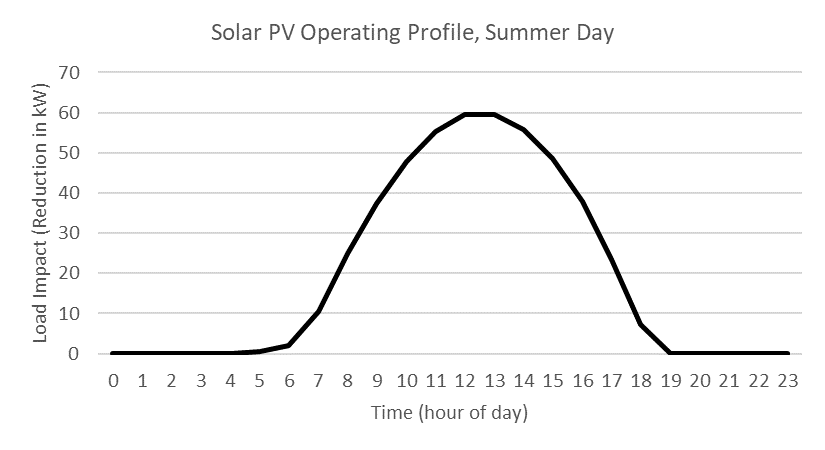 Figure 48. Illustrative example – single DER analysis: simulation of solar PV output for an apartment complex
Source: Smith 2021. Used with permission.
11.4.2. Percent Reductions, Building Simulation Models, and End-Use Load Profiles for Multiple-DER Analysis
Figure 49 shows examples of load impact profiles from a market potential study conducted in 2020 for the State of Hawaii (see AEG 2020). Hawaiian Electric is currently using results from the study to inform its integrated grid planning process. Several scenarios were modeled during the study. The load impacts in Figure 49 represent an “achievable-high” potential scenario, which means cost-effectiveness and likely customer adoption are accounted for in the potential. The profiles reflect hourly load reduction impacts on a critical peak day due to:
- Energy efficiency (EE),
- Demand response / grid services (DR/GS) – for a load shed scenario that includes impacts from electric vehicles (EVs) and other end uses, and
- A time-of-use plus critical peak pricing (TOU+CPP) rate.
The potential was calculated for the year 2030 and includes combined impacts for the residential and commercial sectors.
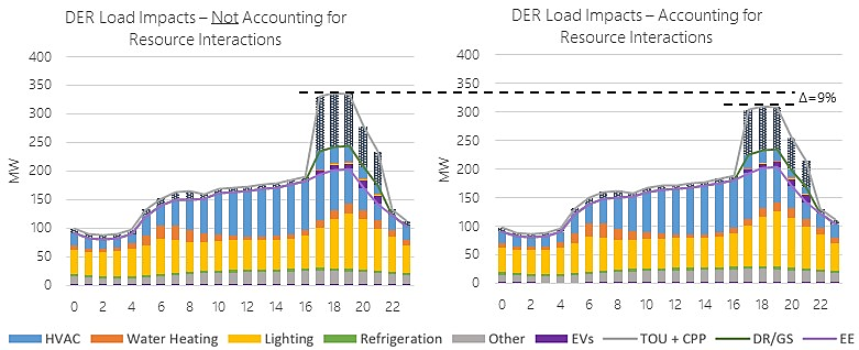 Figure 49. Illustrative example – multiple-DER analysis: comparison of DER load impact profiles with and without accounting for resource interactions
Note: DERs include energy efficiency, demand response (load shed), and TOU+CPP rate. Critical peak day, Oahu, all sectors, 2030. Source: AEG 2020. Used with permission.
The analysis was conducted two ways to depict the effect of resource interactions. First, the DERs were analyzed in isolation to develop impacts that did not account for resource interactions (graph on left in Figure 49). Then, the analysis was revised to account for interactions between the different types of DERs (graph on right in Figure 49). To account for resource interactions, energy efficiency impacts relative to the Reference Case were modeled first. Next, the time-of-use rate was modeled assuming the energy efficiency measures had been implemented.39 Last, the demand response impacts were modeled assuming both the energy efficiency measures and rate were in place. Comparing the two figures shows that the maximum hourly impact was 336 MW (6 pm) for the figure on the left, compared with 309 MW (6 pm) for the figure on the right; this illustrates the point that the load impacts would have been overstated (by about 9 percent for that particular hour) if the resource interactions were not accounted for.
The impacts in Figure 49 were modeled using a combination of the following:
- AEG’s Load Management Analysis and Planning (LoadMAP™) model
- The Brattle Group’s PRISM model
- Building simulation models using Hawaii’s normal weather data for weather-sensitive loads:
- Single-family residential prototypes developed in BEopt™ with EnergyPlus v8.8 as the simulation engine using Hawaii-specific data on housing characteristics and end uses. See Section 11.5.2.a for a description of these simulation models.
- Other building simulations from the NREL’s OpenEI dataset using models developed for IECC Zone 1A, Hawaii’s climate zone. See Section 11.5.1 for a description of NREL’s simulated hourly load profiles.
- End-use load profiles from the California Energy Commission (CEC) for non-weather sensitive measures. See Section 11.5.1 for a description of the CEC’s electricity load profiles.
- The percent reductions approach was used to cast estimates of annual energy efficiency impacts to 8760 hourly end-use profiles.
11.4.3. Constrained Optimization Modeling of Solar PV and Storage
Figure 50 shows an example of results from LBNL’s DER-CAM optimization modeling tool. The tool was used to analyze investment in solar PV and battery storage for a large office building in San Francisco. The model optimized dispatch of the DERs to reduce the customer’s energy costs against a retail tariff with monthly demand charges. The graph in Figure 50 includes the Reference Case load profile (black dashed line labeled “Total Original Electric Load”), the DER Case load profile (green area labeled “Utility Purchase”), PV used by the customer (yellow-orange area), electricity provided by the stationary battery (blue area), and state of charge (S.O.C) of the battery (blue line plotted using axis on right side of graph). The graph depicts electricity dispatch for a peak day in May. Inputs for this model included site data, end-use load data for different day types, utility tariffs and export options, DER options and associated parameters, and optimization objectives and constraints. For more information about this example, see LBNL 2018 DER-CAM.
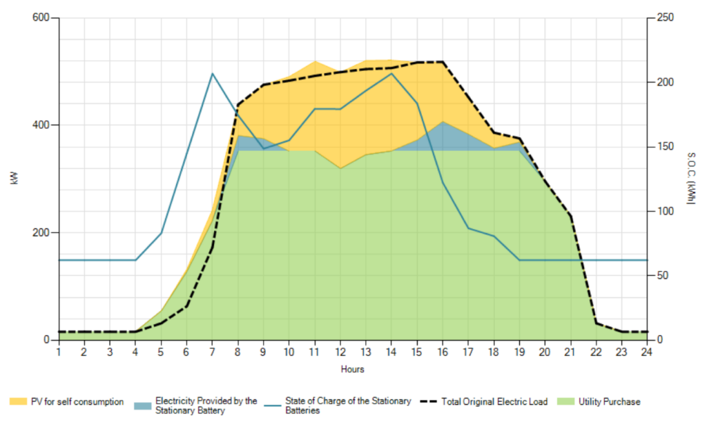 Figure 50. Illustrative example – constrained optimization modeling using DER-CAM
Note: Portrayal of investment in solar PV and battery storage to minimize energy costs for large office building in San Francisco, CA. Source: Grid Integration Group, LBNL 2018 DER-CAM Used with permission.
11.5. Resources for Developing DER Load Profiles
There is a growing library of publicly available tools and resources for developing load and load impact profiles. There are also myriad models and tools that are not public. Figure 51 below provides examples of useful tools and resources in the public domain, with descriptions summarized from information provided on the websites. The major advantages of using existing tools and resources are that they are much simpler, faster, and less expensive to apply. End-use load profile libraries provide load profiles for a wide variety of end-uses, building types, and locations. Some modeling tools for distributed generation and distributed storage allow sensitivity analysis and the ability to readily explore various scenarios without the need for an extensive metering study or pilot program to estimate impacts. Possible concerns with using a tool or resources from a secondary source are the reliability of the underlying information, and the degree to which it is applicable to other services territories with climatic and other regional differences. While some tools and resources allow user input or selection of customized inputs like weather and cost data, others are more limited in their customization features. A key disadvantage of relying solely on public tools and resources is the limited availability of load impact profiles at the end-use level for some types of DER measures and scenarios. However, it is important to note that recent and planned efforts by the national laboratories and others have been mitigating some of these issues.
End-Use Load Profiles
- End-Use Load Profiles for the U.S. Building Stock, NREL, LBNL, Argonne National Laboratory, 2021
- End Use Load Profile Inventory, LBNL, 2019
- California Investor-Owned Utility Electricity Load Shapes, California Energy Commission, 2019
- Commercial and Residential Hourly Load Profiles for all TMY3 Locations in the United States, NREL, 2014
- Load Shape Library, EPRI, version 8.0
Simulation Models
- Building Energy Modeling, DOE
- eQUEST, James J. Hirsch & Associates, Version 3.65
- BEopt™, NREL, Version 2.8.0.0,
- PVWatts® Calculator, NREL, version 6.2.4
Optimization Models
- SAM: System Advisory Model, NREL, version 2020.2.29
- REopt™ Lite, NREL, version Feb 2021
- DER-CAM, LBNL
- QuESt, Sandia National Laboratories
- Storage Value Estimation Tool (StorageVET® 2.1), EPRI
- DER Value Estimation Tool (DER-VET™), EPRI
- HOMER Grid and HOMER Pro, Homer Energy
Normalized Metered Energy Consumption
- OpenEEmeter, Recurve and LF Energy
Impact Estimation References
- CalTRACK, Working Group under Energy Market Methods Consortium (EM2)
- IPMVP, Efficiency Valuation Organization
- Uniform Methods Project, DOE Office of Energy Efficiency & Renewable Energy
Figure 51. Examples of publicly available tools and resources for developing load and load impact profiles
11.5.1. End-Use Load Profiles
- End-Use Load Profiles for the U.S. Building Stock, NREL, LBNL, Argonne National Laboratory, 2021 (www.nrel.gov/buildings/end-use-load-profiles.html) – Database of end-use load profiles representing all major end uses, building types, and climate regions in the U.S. commercial and residential building stock. Developed with simulation models calibrated and validated with empirical datasets. The output of each building energy model is 1 year of energy consumption in 15-minute intervals, separated into end-use categories. The dataset has also been formatted to be accessible in three ways—via pre-aggregated load profiles in downloadable spreadsheets, a web viewer, and a detailed format that can be queried with big data tools—to meet the needs of many different users and use cases.
- End Use Load Profile Inventory, LBNL, 2019 (www.emp.lbl.gov/publications/end-use-load-profile-inventory) – An Excel file that lists datasets that contain hourly load profiles and are publicly available. The inventory includes load profile data from submetering, master metering, and plug loads. Metadata about each data source is recorded, in an effort to aid researchers looking for existing load profile studies and wishing to filter by attributes such as location, customer sector, or end-use category.
- California Investor-Owned Utility Electricity Load Shapes, California Energy Commission, 2019 (www.energy.ca.gov/publications/2019/california-investor-owned-utility-electricity-load-shapes) – This project updated traditional end-use load shapes for six energy sectors and developed photovoltaic system, light-duty electric vehicle, and energy efficiency load impact profiles, which will be used as inputs for the Demand Analysis Office’s California Energy Demand Forecast. The California Energy Commission currently uses the Hourly Electric Load Model to cast annual energy demand forecast elements into hourly demands, from which projected annual peak loads are forecasted. The Hourly Electric Load Model includes weather-sensitive and weather-insensitive load shapes at the end-use, planning area, and forecast zone level for the residential and commercial sectors, and at the whole-building level for other sectors. The project updated end-use load shapes by blending publicly available load shapes from market and metering studies with building simulations in a framework known as EnergyPlus. The project relied on aggregated interval meter data provided by electric investor-owned utilities to calibrate energy simulations and to develop models for other sectors. The load shapes and profiles developed under this project are dynamic entities within “load shape generators,” which can respond to relevant factors such as calendar data, weather data, macroeconomic data, and in some cases, price signals from utility time of use rates.
- Commercial and Residential Hourly Load Profiles for all TMY3 Locations in the United States, NREL, 2014 (www.data.openei.org/submissions/153) – Hourly end-use load profile data for 16 commercial building types and residential buildings in all TMY3 locations in the United States. The commercial load data is based on the Commercial Reference Buildings (www.energy.gov/eere/buildings/commercial-reference-buildings) and the residential load is based on the Building America House Simulation Protocols (www.nrel.gov/docs/fy11osti/49246.pdf).
- Load Shape Library, EPRI, version 8.0 (www.loadshape.epri.com/) – Intended to demonstrate basic features of Load Shape Profiling. Website has interactive interface to view hourly end-use load shapes by sector and whole premise load shapes by building type and sector. There are also some hourly and daily load shapes for certain residential measures by location, day type, and technology type.
11.5.2. Models
11.5.2.a. Simulation Models
- Building Energy Modeling, DOE (www.energy.gov/eere/buildings/about-building-energy-modeling) – Through the Building Technologies Office (BTO), DOE develops and maintains two software packages for building energy modeling: EnergyPlus™ (version 9.3.0) and OpenStudio™. EnergyPlus is an open-source whole-building energy modeling engine; it is the successor to the DOE-2 (version 2.1E) simulation engine developed by LBNL. OpenStudio is a software development kit that reduces the effort of EnergyPlus-based application development. BTO distributes EnergyPlus and OpenStudio under a commercial-friendly non-exclusive open-source license.
- eQUEST, James J. Hirsch & Associates, Version 3.65, (www.doe2.com/equest/) – The QUick Energy Simulation Tool (eQuest) is a free user-interface that combines schematic and design development building creation wizards, an energy efficiency measure wizard and a graphical results display module with the DOE-2 (version 2.2) building energy use simulation program.
- BEopt™, NREL, Version 2.8.0.0, (www.nrel.gov/buildings/beopt.html) – The BEopt (Building Energy Optimization Tool) software is free. It provides capabilities to evaluate residential building designs and identify cost-optimal efficiency packages at various levels of whole-house energy savings along the path to zero net energy. It can be used to analyze both new construction and existing home retrofits, as well as single-family detached and multi-family buildings, through evaluation of single building designs, parametric sweeps, and cost-based optimizations. It provides detailed simulation-based analysis based on specific house characteristics, such as size, architecture, occupancy, vintage, location, and utility rates. Discrete envelope and equipment options, reflecting realistic construction materials and practices, are evaluated. BEopt uses the EnergyPlus simulation engine.
- PVWatts® Calculator, NREL, version 6.2.4 (www.pvwatts.nrel.gov/) – PVWatts is a free, basic solar modeling tool that estimates energy production and costs of grid-connected PV systems. It calculates hourly or monthly PV energy production based on minimal inputs and can be used to develop generation profiles. An online interactive interface utilizes the PVWatts calculator.
11.5.2.b. Optimization Models
- SAM: System Advisory Model, NREL, version 2020.2.29 (www.sam.nrel.gov/) – SAM is a free tool that models techno-economic performance and cost predictions of renewable energy systems, including distributed PV, battery storage, wind power, and other types of distributed renewable energy systems.
- REopt™ Lite,NREL, version Feb 2021 (www.reopt.nrel.gov/tool) – REopt Lite is a free web-based tool for evaluating the economic viability of distributed PV, wind, battery storage, combined heat and power, thermal energy storage, and geothermal heat pumps (GHP) at an existing site. It identifies system sizes and dispatch strategies to minimize energy costs. It also estimates how long a system can sustain critical load during a grid outage.
- DER-CAM, LBNL (www.gridintegration.lbl.gov/der-cam) – The Distributed Energy Resources Customer Adoption Model (DER-CAM) is a free decision support tool that can be used to find the optimal portfolio, sizing, placement, and dispatch of a wide range of DERs in the context of either buildings or multi-energy microgrids, while co-optimizing multiple stacked value streams that include load shifting, peak shaving, power export agreements, or participation in ancillary service markets. While the objective function of DER-CAM can be easily modified — or even replaced by a multi-objective analysis — it is most commonly defined as a site’s total annual cost of energy supply. This includes costs associated with both new and existing DER, operation and maintenance costs, fuel costs, and also all costs related to utility imports either fixed, time-dependent, energy-based, or power-based. Additionally, all value streams associated with the optimal DER dispatch determined by DER-CAM are considered in the objective function, both in the form of avoided costs and market participation. The model requires hourly end-use profiles as inputs and provides outputs of when and how the DER should optimally be dispatched. See LBNL 2018 DER-CAM for steps to complete a DER-CAM analysis.
- QuESt, Sandia National Laboratories (www.sandia.gov/ess-ssl/tools/quest/) – QuESt is a free, open source, application suite for energy storage simulation and analysis. It currently consists of three applications that help project users evaluate energy storage systems for different use cases. QuESt Data Manager helps manage the acquisition of ISO market data, US utility rate data, commercial and residential load profiles, and essential data for use in other QuESt applications. Given an energy storage device, an electricity market with a certain payment structure, and market data, QuESt Valuation estimates the maximum revenue from participating in energy arbitrage or providing ancillary services. QuESt BTM estimates cost savings from behind-the-meter energy storage for time-of-use and net energy metering customers. A PV power profile can be included to co-locate with a building and energy storage. It uses a location-specific commercial and residential building load profile from secondary open sources to represent demand and provides monthly estimates of cost savings.
- Storage Value Estimation Tool (StorageVET® 2.1), EPRI (www.storagevet.com) – StorageVET 2.1 is a free, web-hosted, energy storage value simulation tool. It facilitates the understanding of where to place and install energy storage, the optimum size as well as controls options. It implements dispatch optimization with sensitivity analysis to assist in planning energy storage project development by enabling rapid analysis of scenarios with different storage sizes, costs, and value streams. Additionally, StorageVET 2.1 is valuable as a research tool to inform broad-sweeping analyses of trends in storage value as a function of location, operation, and technical capabilities.
- DER Value Estimation Tool (DER-VET™), EPRI (www.der-vet.com) – DER-VET is a free, open-source, optimization-based energy valuation and planning tool for DERs and larger, centralized energy resources. It was developed by expanding on the framework developed in EPRI’s Storage Value Estimation Tool (StorageVET). It supports site-specific assessments of energy storage and additional DER technologies—including solar, wind, demand response, electric vehicle charging, internal combustion engines, and combined heat and power—in different configurations, such as microgrids. It uses load and other data to determine optimal size, duration, and other characteristics for maximizing benefits based on site conditions and the value that can be extracted from targeted use cases.
- HOMER Grid and HOMER Pro, Homer Energy (www.homerenergy.com/) – HOMER Grid combines engineering and economics to rapidly perform complex calculations for comparing design outcomes and considering options for minimizing project risk and reducing energy expenditures. It allows for any combination of components (electric vehicle charging, battery, solar, wind, generator, grid, combined heat and power) and outputs the total energy cost for each possible system. The optimization features allow for maximizing savings, minimizing cost, increasing resilience, optimizing electric vehicle charging stations, reducing carbon emissions, stacking values to increase return on investment, and exploring combined heat and power. HOMER Pro simulates the operation of a hybrid microgrid for an entire year, in time-steps from one minute to one hour. It looks at all possible combinations of equipment and presents options that can be selected to create an optimal system. Both of these models provide tools to help the user select and customize load profiles. The outputs from HOMER Pro include hourly time series plots for viewing the generation from each component, how it serves the load, the resources that power the components, as well as a number of key operational characteristics from each component for an entire year of your simulation. There is also a “profile” option that shows the hourly performance for an average day for each month for the selected parameter.
11.5.2.c. Normalized Metered Energy Consumption
- OpenEEmeter, Recurve and LF Energy (www.lfenergy.org/projects/openeemeter/) – An open source toolkit for implementing and developing standard methods for calculating normalized metered energy consumption (NMEC) and avoided energy use. The OpenEEmeter library contains routines for estimating energy efficiency savings at the meter. OpenEEmeter includes the reference implementation of the CalTRACK methods (see below) for estimating normalized metered energy savings. OpenEEmeter, as implemented in the eemeter package and its companion eeweather package, contains the most complete open source implementation of the CalTRACK methods, which specify a family of ways to calculate and aggregate estimates of avoided energy use at a single meter particularly suitable for use in pay-for-performance programs. The model does not directly generate load profiles, but can be used with reference case and DER case load data to generate profiles.
11.5.3. Impact Estimation Resources
- CalTRACK, Working Group under Energy Market Methods Consortium (EM2) (www.caltrack.org/) – CalTRACK specifies a set of empirically tested methods to standardize the way normalized meter-based changes in energy consumption are measured and reported. When CalTRACK is implemented through open source software, these methods can be used to support procurement of energy efficiency, electrification, and other DERs.
- IPMVP, Efficiency Valuation Organization (www.evo-world.org/en/products-services-mainmenu-en/protocols/ipmvp) – The International Performance Measurement and Verification Protocol (IPMVP) provides methods, with different levels of cost and accuracy, for determining savings either for the whole facility or for individual energy conservation measures.
- Uniform Methods Project, DOE Office of Energy Efficiency & Renewable Energy (www.energy.gov/eere/about-us/ump-home) – Under the Uniform Methods Project, DOE is developing a set of protocols for determining savings from energy efficiency measures and programs. The protocols provide a straightforward method for evaluating gross energy savings for residential, commercial, and industrial measures commonly offered in ratepayer-funded programs in the United States. The measure protocols are based on a particular International Performance Verification and Measurement Protocol (IPMVP) option but provide a more detailed approach to implementing that option.
11.5.4. Resources for Developing DER Load Profiles
Amara-Ouali, Y., Goude, Y., Massart, P., Poggi, Je., Yan, H. 2021. “A Review of Electric Vehicle Load Open Data and Models.” Energies 2021, 14, 2233. doi.org/10.3390/en14082233.
Applied Energy Group. 2017. (AEG 2017). Marrin, K., Shah, T. and Williams, T., Pacific Gas & Electric Company’s SmartMeter™ Enabled Programs: Program Year 2016 Evaluation of Customer Web Presentment and Bill Forecast Alert, Apr 2017, CALMAC ID PGE0379.01.
Applied Energy Group. 2018. (AEG 2018). Marrin, K., Parmenter, K., Duer, A., Nguyen, A. and Shah, T., 2017 Statewide Load Impact Evaluation of California Aggregator Demand Response Programs, Applied Energy Group, Apr 2018, CALMAC ID PGE0410.01.
Applied Energy Group. 2020. (AEG 2020). Rohmund, I., Parmenter, K., Kolnowski, K. (AEG), State of Hawaii Market Potential Study, Prepared for the Hawaii Public Utilities Commission, Applied Energy Group, Jul 2020, www.hawaiienergy.com/images/about/information-and-reports/market-potential-study/mps_state-of-hawaii-market-potential-study-2020.pdf.
California Independent System Operator. 2021. (CAISO 2021). Demand Response Advancement Measurement Methodology: Analysis of Open-Source Baseline Comparison Group Methods to Enable CAISO Demand Response Resource Performance Evaluation. J. Glass, S. Suffian, A. Scheer, C. Best. November. http://www.caiso.com/Documents/DemandResponseAdvancedMeasurementMethodology.pdf
Electric Power Research Institute 2018. (EPRI 2018). Electric Vehicle Driving, Charging, and Load Shape Analysis: A Deep Dive into Where, When, and How Much Salt River Project (SRP) Electric Vehicle Customers Charge, Palo Alto, CA: 3002013754.
Lawrence Berkeley National Laboratory. 1990. (LBNL 1990). Eto, J.H., Akbari, H., Pratt, R.G. and Braithwait, S.D., “End-Use Load Shape Data Application, Estimation, and Collection: A State-of-the-Art Review,” Presented at the ACEEE 1990 Summer Study on Energy Efficiency in Buildings, Pacific Grove, CA, Aug 26 – Sep 1, 1990, Prepared for the U.S. Department of Energy under Contract Number DE-AC03-76SF00098, eta-publications.lbl.gov/sites/default/files/lbnl-30141.pdf.
Lawrence Berkeley National Laboratory. 2018. (LBNL 2018 DER-CAM). “Modeling Workflow: Completing a DER-CAM analysis in 7 steps,” Presentation, March 7, 2018, www.gridintegration.lbl.gov/sites/default/files/DER-CAM%20Workflow.pdf.
Lawrence Berkeley National Laboratory. 2020. (LBNL 2020 EE-DR). Andrew J. Satchwell, A.J., Peter A. Cappers, P.A., Jeff Deason, J., Sydney P. Forrester, S.P., Natalie Mims Frick, N., Brian F. Gerke, B.F. and Mary Ann Piette., M.A., A Conceptual Framework to Describe Energy Efficiency and Demand Response Interactions. July 2020, eta-publications.lbl.gov/sites/default/files/lbnl_report_ee_and_dr_interactions_framework_final_posted.pdf
Lawrence Berkeley National Laboratory. 2020. (LBNL 2020 EE Buildings). Gerke, B.F., Zhang, C., Satchwell, A., Murthy, S. and Piette, M.A., Lawrence Berkeley National Laboratory; Present, E., Wilson, E., Speake, A. and Adhikari, R., “Modeling the Interaction Between Energy Efficiency and Demand Response on Regional Grid Scales,” 2020 ACEEE Summer Study on Energy Efficiency in Buildings, Aug 2020, eta-publications.lbl.gov/sites/default/files/gerke_aceee_paper_pre-print.pdf.
Lawrence Berkeley National Laboratory. 2021. (LBNL 2021 Hourly Savings). Murphy, S., Deason, J. and Satchwell, A. “Timed to save: the added value of accounting for hourly incidence of electricity savings from residential space-conditioning measures.” Energy Efficiency 14, 82. doi.org/10.1007/s12053-021-09994-5.
Lawrence Berkeley National Laboratory. 2022 (LBNL 2022). Time Sensitive Value Calculator for Energy Efficiency and Other Distributed Energy Resources: Users Guide. Natalie Mims Frick, J. Carvallo, M. Pigman. February. https://eta-publications.lbl.gov/sites/default/files/tsv_user_manual_v6_0.pdf
Nguyen, T.A., Byrne, R.H. 2021. “Software Tools for Energy Storage Valuation and Design,” Current Sustainable/Renewable Energy Reports 8, 156–163, doi.org/10.1007/s40518-021-00186-4.
Rocky Mountain Institute. 2018. (RMI 2018 NWS). The Non-Wires Solutions Implementation Playbook, A Practical Guide for Regulators, Utilities, and Developers. Dyson, M., Prince, J., Shwisberg, L. and Waller, J. rmi.org/wp-content/uploads/2018/12/rmi-non-wires-solutions-playbook-report-2018.pdf.
Smith, C.B. and Parmenter, K. 2021. Use of NREL’s PVWatts® calculator to model a solar PV system at a senior living facility. Unpublished.
State and Local Energy Efficiency Action Network. 2020. (SEE Action 2020). Performance Assessments of Demand Flexibility from Grid-Interactive Efficient Buildings: Issues and Considerations. Schiller, S.R., Schwartz, L., and Murphy, S., Lawrence Berkeley National Laboratory. emp.lbl.gov/publications/performance-assessments-demand.
28 Use of the term “load impact profile” is common for energy efficiency, electrification, and demand response resources, while “operating profile” is more commonly used for distributed generation and distributed storage.
29 This handbook uses “one DER” or “single DER” to refer to one type of DER being analyzed for a group of customers.
30 Can capture the combined impact of multiple DERs, but it is difficult to allocate impacts to individual DERs.
31 A 1990 ACEEE publication refers to many of these same methods (see LBNL 1990).
32 When a sample of buildings is being simulated to represent a population of buildings, an additional calibration step can be performed. First, expand simulated loads for the sample to the population. Then make adjustments to reconcile the simulated values with the metered loads for the population.
33 See AEG 2017 for an example of using both the difference-in-differences approach and the fixed effects regression approach to estimate load impacts for SmartMeter-enabled informational energy efficiency programs.
34 See LBNL 2021 Hourly Savings for an example of using regression analysis to estimate hourly load impacts from residential space conditioning measures.
35 See AEG 2018 for an example of using customer-specific regression analysis to estimate hourly load impacts for aggregator-based demand response programs.
36 Additional steps may be required to create a matched control group if the control group has not already been defined.
37 See SEE Action 2020 for more information issues and considerations related to assessing impacts from grid-interactive efficient buildings. See RMI 2018 NWS for more information on implementing non-wires solutions.
38 Line losses for distributed generation are likely to be inconsequential.
39 For visual clarity, impacts for the rate appear on the top of the load impact profile with the black and white cross pattern and the gray line, even though the rate was second in the loading order.