3.2. Generation Impacts
3.2.1. Energy Generation
3.2.1.a. Definition
Energy generation costs consist of the fuel and variable O&M costs from the production or procurement of energy (i.e., kWh) from generation resources. Energy generation costs can vary significantly by season and time of day. Figure 5 presents the variability of locational marginal energy prices in ISO New England throughout a year, tracked in real time throughout 2021.
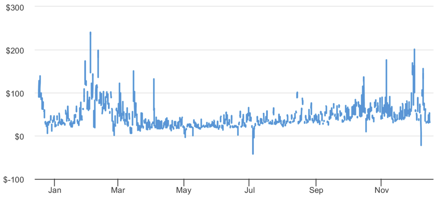 Figure 5. Daily locational marginal price at New England Hub ($/MWh)
Source: U.S. Energy Information Administration. 2021. “New England Dashboard.” (Accessed 12/17/2021). Available at: www.eia.gov/dashboard/newengland/electricity.
In general, DERs will (a) create energy generation benefits when they reduce the amount of electricity utilities need to produce or procure in order to meet load, or (b) create energy generation costs if they require higher levels of energy generation. An exception to this occurs during periods of negative pricing whereby consuming grid energy (e.g., storage or electric vehicle charging) results in a benefit and curtailing grid energy consumption results in a cost.
3.2.1.b. Methods for Calculating Energy Generation Impacts
Figure 6 summarizes the common methods for estimating energy generation impacts, each of which is described in detail below. Section 3.2.1.c further summarizes the advantages and disadvantages of each method (see Table 12).
Proxy Unit Method
- Determine energy saved or generated using DER load impact profile
- Identify proxy unit(s) to be avoided ·Identify proxy unit operating costs to determine avoided energy costs
- Escalate costs over study period
Power Sector Modeling
- Develop Reference Case forecast for meeting load
- Run capacity expansion model to determine future resource build-out
- Simulate dispatch of resources using production cost model to determine energy prices for single year
- Extend production cost modeling over BCA study period
Market Data Method
- Determine energy saved or generated using DER load impact profile
- Obtain historical LMPs from system operator website
- Calculate avoided energy costs by weighting LMPs by the load impact profile of the DER or DER portfolio
- Escalate avoided energy costs over study period
Public and Proprietary Forecasts
- Use publicly available historical energy cost data as benchmark
- Use publicly available forecasts as inputs
- Obtain proprietary energy generation impact forecasts to use as inputs, if possible
Figure 6. Common methods for estimating energy generation impacts
Option 1: Proxy Unit Method
The proxy unit method calculates the energy generation impacts associated with a hypothetical generation unit that would be avoidable by the procurement of DERs (see EPA 2018; NREL 2014 DPV). The proxy unit should represent the generation resource likely to be on the margin during the time of day a DER impact would occur.
This method is one of the more simplistic approaches to calculating avoided energy generation costs. It involves the key steps shown in Table 6.
Table 6. Steps for using the proxy unit method for determining energy generation impacts
| Step 1
|
Determine the energy saved or generated by the proposed DER
This can be determined using the proposed DERs’ load impact profiles (see Chapter 11). Ideally, the savings or generation would be developed on an hourly basis, to reflect the variation across different time periods.
|
| Step 2
|
Identify the proxy unit that will be avoided by the DERs
Use the load impact profile of the DERs from Step 1 to establish which generation unit is likely to be on the margin at the time of DER operation and should therefore serve as the proxy unit. For example, energy efficiency is more likely to impact baseload generation on a system, indicating that the marginal unit would likely be a coal plant or natural gas combined cycle plant. Whereas storage is typically operated on-peak and will impact peaking resources like a natural gas combustion turbine plant.
If the portfolio of DERs has a wide range of load impact profiles, more than one proxy unit may be identified. In this situation, a weighted proxy unit can be calculated based on weighting multiple proxy units by the DER load impact profiles.
|
| Step 3
|
Identify the operating costs of the proxy unit
This will include fuel costs (e.g., natural gas or oil), variable O&M costs (i.e., costs that are a function of energy generation), and marginal emissions costs that are embedded in the cost of generation. The operating costs of the proxy unit will serve as the energy generation impacts of the DER.
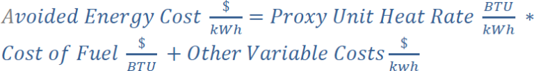
The calculation for avoided energy generation costs using the Proxy Unit Method is:
|
| Step 4
|
Escalate avoided energy costs from Step 3 over the study period
The fuel cost portion can be escalated using fuel price forecasts. The other variable costs can be escalated using real escalation factors associated with electricity and gas costs.
|
The primary advantages of this method include its simplicity and use of generic, public data. The primary disadvantages include its potential inaccuracy if the selected proxy unit does not accurately reflect the operating characteristics of the DERs. Further, it does not capture the potential impacts to baseload units, and it does not account for future changes to the electric system that may lead to changes in the marginal unit.
Key Data Sources for Proxy Unit Method
Data for determining operating costs for the proxy unit is available from the following sources.
- Electricity and natural gas price forecasts
- U.S. EIA’s Annual Energy Outlook. (See U.S. EIA AEO 2022.)
- New York Mercantile Exchange gas futures. (See CME Group, Henry Hub.)
- Horizons Energy’s National Database. (See Horizons Energy, n.d.)
- NREL’s annual technology baseline has heat rates and projected variable O&M costs for various types of electrical generators. (See NREL ATB.)
- Marginal fuel mix can often be found on ISO and RTO websites. (See PJM Fuel Data.)
Option 2: Power Sector Modeling Method
Power sector modeling tools are a detailed and complex approach to calculating energy generation impacts. The most common tools are the capacity expansion model and the production cost model, described in Figure 7 below.
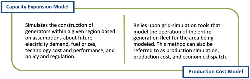 Figure 7. Summary description of capacity expansion and production cost models
A production cost model typically provides for higher temporal resolution (i.e., hours to minutes) than the capacity expansion model. However, a production cost model will only report short-run impacts, unless it is paired with a capacity expansion model. Therefore, the production cost model is typically used in combination with a capacity expansion model to develop long-run avoided energy generation costs.
The use of the capacity expansion with the production cost model for developing energy generation impacts typically involves the steps in Table 7.
Table 7. Steps for developing energy generation impacts with capacity expansion and production cost modeling
| Step 1
|
Develop a Reference Case forecast for how load will be met
This forecast should include the customer load expected over the study period but should not include the load impacts of the DERs being evaluated in the BCA (see Section 2.5). This involves entering the following inputs into the model: the projected growth in electricity demand, changes in energy and fuel prices, existing fleet of generating assets, operating characteristics of potential new generating units, and environmental regulations (current and planned). The capacity expansion model uses these inputs to determine a future business-as-usual build-out of the system through an optimization process that chooses the least-cost solution to adding capacity.
|
| Step 2
|
Run the capacity expansion model
This process will determine the future resource build-out on the system.
|
| Step 3
|
Run the production cost model
Using the resource build-out from Step 2, the production cost model should be run to simulate the dispatch of those resources. The model will determine the least-cost mix of generators needed to meet load during a given time interval, typically one year in 8,760-hour increments. The production cost model will output the avoided energy cost in the form of energy prices.
|
| Step 4
|
Forecast energy costs over the BCA study period
Production cost models typically provide one-years’ worth of energy costs. Calculating energy costs over the BCA study period requires running a production cost model for multiple years to capture the changing generator mix over time, based on the results of the capacity expansion model. For practical purposes, the production cost model runs can be limited, for example by running it for the first 10 years and extrapolating beyond that, or by running it in five-year intervals and interpolating between them.
|
(See U.S. DOE Gateway; NREL 2014 DPV.)
Table 8 below provides information on a range of capacity expansion and production cost models available for analyzing energy generation impacts.
Table 8. Examples of capacity expansion and production cost models to estimate energy generation impacts
Note: *Model can be used in Production Cost and Capacity Expansion mode. The utility-scale models often have higher spatial and temporal resolution and are often used for IRPs (See U.S. DOE Gateway).
Key Data Sources for Power Sector Models
The capacity expansion and production cost models require significant data collection. This includes fuel price forecasts, load forecasts, transmission constraints, electricity generator cost and performance assumptions for both existing and potential new plants, DER cost and performance assumptions (including load impact profile), and state and federal environmental regulations and requirements (see NREL 2014 RPS.)
To populate the needed inputs, databases for models are available for purchase but require technical expertise. In some models, default data may be included, but modifying this data to fit the needs of the analysis may require technical expertise.
Some models calibrate historical or projected results against other existing datasets, such as the NEMS-generated Annual Energy Outlook produced by U.S. EIA, or historical data published by U.S. EIA or independent system operators. In other cases, this calibration is left up to the user to do on their own.
Data for individual power plants is available from public sources:
- Capacity and average heat rate data:
- FERC forms 1 and 714
- U.S. EIA 2020
- Part-load heat rate data must be obtained from the operator or by reconstructing them via U.S. Environmental Protection Agency (EPA) historical continuous emissions monitoring system (CEMS) datasets. (See NREL 2014 RPS.)
Table 9 provides multiple examples of how states use power sector models to analyze energy generation impacts.
Table 9. State examples using the power sector model method to estimate energy generation impacts
| State
|
Summary
|
| New England states
|
2021 AESC projects New England electric system energy levels and prices from 2021 to 2035 using the EnCompass model (in both capacity expansion and production cost mode). The wholesale energy prices produced by the model change over time (and on a peak and off-peak basis) depending on the system demand, available units, transmission constraints, fuel prices, and other attributes. (See AESC 2021.)
|
| California
|
California Public Utilities Commission (CPUC) uses SERVM, “a production simulation model that represents a theorized and optimized view of the day-ahead market” to develop avoided energy costs for DERs. SERVM generates wholesale electricity prices based on the input system load and dispatch of the modeled generation portfolio. (See CPUC 2020.)
|
| Georgia
|
Southern Company uses an hourly production cost model to develop its avoided energy costs. The model uses scenario-specific information including fuel price forecasts, fleet expansion plans, and emissions allowance prices. The model also includes inputs related to unit characteristic like heat rates, emission rates, and variable O&M, as well as transmission constraints, and economic energy purchases and sales. (See Southern Company 2017.)
|
| South Carolina
|
The marginal value of energy derived from production simulation runs per the utility’s most recent IRP study and/or Public Utility Regulatory Policy Act (PURPA) Avoided Cost formulation. (See E3 2015.)
|
| North Dakota
|
Black Hills used a production cost model to determine the hourly costs of serving its system load of a 20-year contract for a Qualifying Facility (QF). The production cost model forecasts the hourly dispatch of the dispatchable resources based on how the marginal production cost of each resource compares to the market price in each hour. (See White 2019.)
|
Option 3: Market Data Method
In restructured markets, avoided energy generation impacts can be based on wholesale market prices. These prices are based on what generators bid into the market and represent the actual costs for operating marginal units. This is a relatively simplistic method that only requires the use of a spreadsheet to calculate energy generation impacts.
Within these markets, it is common to use the Locational Marginal Price (LMP) that can be obtained for specific points (nodes) on the system. LMPs can also be obtained for on-peak and off-peak periods, hourly, and in some cases for five-minute intervals. Depending upon the Independent System Operator (ISO), LMPs can include energy costs, capacity costs, and transmission congestion costs. Therefore, it is important to ensure that the energy generation impacts are not double-counting capacity or transmission impacts.
Calculating energy generation impacts using this method involves the four key steps shown in Table 10.
Table 10. Steps for calculating energy generation impacts using the market data method
| Step 1
|
Determine the energy saved or generated by the proposed DER
This can be determined using the proposed DERs’ load impact profiles (see Chapter 11). Ideally, the savings or generation would be developed on an hourly basis, to reflect the variation across different time periods.
|
| Step 2
|
Obtain historical LMPs from the system operator’s website
This information is available to the public. Depending on the age of the data it may need to be adjusted for inflation.
|
| Step 3
|
Calculate the avoided energy cost
Weight the LMPs by the load impact profile of the DER or DER portfolio.
|
| Step 4
|
Escalate avoided energy costs from Step 3 over the study period
Some markets like NYISO provide annual and hourly forecasts of LMP for 20 years. However, other markets like MISO, PJM, and ISO-NE do not provide public forecasts. In these cases, prices can be escalated using forecasts from publicly available sources. (See U.S. EIA AEO 2022.)
|
(See RAP 2013; ConEdison 2020; NREL 2014 RPS; Clean Power Research 2015.)
Key Data Sources for Market Data Method
The following sources provide useful information for escalating energy costs:
- U.S. EIA’s Annual Energy Outlook. (See U.S. EIA AEO 2022.)
- New York Mercantile Exchange (NYMEX) gas futures is applicable for systems that are driven by natural gas generation resources (e.g., ISO-NE, PJM). (See CME Group, Henry Hub.)
- Horizons Energy’s National Database. (See Horizons Energy, n.d.)
- Market and system operator hourly marginal costs. (See FERC Form 714.)
For examples of states using the market data method to estimate energy generation impacts, see Table 11 below.
Table 11. State examples using the market data method to estimate energy generation impacts
| State
|
Summary
|
| Arkansas
|
Uses MISO LMPs weighted by a standard output of a DER then escalated using the long-term forecast of natural gas prices from U.S. EIA’s Annual Energy Outlook at the Henry Hub. (See Crossborder Energy 2017.)
|
| New York
|
NYISO provides annual and hourly locational-based marginal price (LBMP) forecasts for 20 years by zone for bulk system, which accounts for energy, congestion, and losses. Hourly LBMP is then applied to the energy associated with the DER load impact profile, adjusted for losses. (See ConEdison 2020.)
|
| Washington D.C.
|
For solar, uses LMPs (minus congestion and marginal loss costs) for the PEPCO zone of PJM. The total avoided energy benefit across each year is calculated by correlating each hour’s generation in PVWatts to a system marginal energy cost, based on historical data for the PJM Interconnect. For future years, U.S. EIA’s Annual Energy Outlook Reference Case was used to scale up the base-year weighted energy cost, based on generation prices in the relevant PJM region. (See Synapse 2017.)
|
| New Jersey
|
Calculated using the three-year rolling average of historical PJM wholesale prices multiplied by the quantity of electricity not consumed. (See NJ BPU 2020.)
|
Option 4: Publicly Available Energy Generation Impacts
It is sometimes possible to use energy generation impacts provided by publicly available sources, instead of the methods described above. For example, when regional studies are prepared for multiple states or when the available forecasts are suitable for the level of detail needed for the DER BCA. The following is a list of publicly available data sources.
Historical Information
Historical energy cost data cannot be directly used as inputs for forward-looking BCAs. Nonetheless, historical energy cost data might be helpful as a starting point for developing forecasts or as a benchmark against which to evaluate forecasts.
- Hourly marginal energy costs. (See FERC Form 714.)
- DOE’s State and Local Energy Data (SLED) provides basic energy market information including electricity generation, fuel sources and costs, applicable policies, regulations, and financial incentives. (See OpenEI State and Local.)
- National Electric Energy Data System (NEEDS) is the database of existing and planned-committed generating units used to construct the “model” plants in U.S. EPA’s current base case of the IPM Model. It specifies plant characteristics including capacity, heat rate, and emissions rates. (See U.S. EPA NEEDS.)
- System lambdas: for jurisdictions with vertically integrated utilities, system lambdas can be used. The system lambda represents the marginal cost of electricity in a system (i.e., the marginal cost of the marginal unit). This approach may underestimate costs due to the fact it does not account for marginal transmission losses, congestion costs, or scarcity prices during constrained hours. (See FERC Form 714.)
Forecasts
- Avoided Energy Supply Components in New England: 2021 Report provides avoided energy generation impacts for the six New England States. (See AESC 2021.)
- California Avoided Cost Calculator provides avoided energy generation impacts for DERs deployed in the state of California. (See CPUC 2020 Avoided Costs; E3 EE.)
- Northwest Power and Conservation Council (NPCC) for Idaho, Montana, Oregon, and Washington provides a wholesale electricity price forecast and its Production Cost Simulation results. (See NPCC Forecast; NOCC Production Cost Simulation).
Option 5: Proprietary Energy Generation Impact Forecasts
Utility forecasts are often proprietary. Typically, the only way for non-utility stakeholders to obtain proprietary forecasts is through a docketed case where discovery is permitted.
There are also for-profit companies that develop and provide forecasts for a fee. Examples include, Wood Mackenzie, HIS Global, and Bentek.
3.2.1.c. Choosing a Method to Calculate Energy Generation Impacts
Table 12 provides a summary of common methods for estimating avoided energy generation impacts with a brief description of the method, its advantages, and disadvantages.
Table 12. Advantages and disadvantages of common methods to calculate energy generation impacts
| Method
|
Description
|
Advantages
|
Disadvantages
|
| Proxy Unit
|
Calculates the energy generation impacts associated with a hypothetical generation unit that would be avoidable by the procurement of DERs
|
Simple approach; information available to those outside of utility; does not require detailed data or modeling; inexpensive
|
May produce inaccurate costs; may not apply to DERS with vastly different load impact profiles; does not reflect displacement of baseload units or changes to system over time; may miss interactive effects
|
| Power Sector Modeling
|
Capacity Expansion model and Production Cost model
|
Provides granular pricing (hourly and sub-hourly); high level of accuracy due to ability to capture complex interactions, variable costs, and generation dispatch characteristics
|
Requires technical expertise and is labor intensive and expensive; lack of transparency and information asymmetry between utilities and stakeholders
|
| Market Data
|
Uses wholesale electricity prices, which reflect the actual costs for operating marginal units in the bids that generators submit; uses system lambdas for vertically integrated utilities
|
Relatively simple approach; captures regional variation; based on local generation mix; includes transmission congestion
|
Potential to double-count impacts with other avoided costs; susceptible to weather misalignment
|
| Public and Proprietary Forecasts
|
Use publicly available historical energy cost data as benchmark for making forecasts; use publicly available or proprietary forecasts as inputs
|
Simple approach; information available to those outside of utility; does not require detailed data or modeling; inexpensive
|
May not be as granular as desired; may not be as accurate or as up-to-date as other methods; proprietary forecasts might be expensive or unavailable to some stakeholders
|
3.2.1.d. Resources for Calculating Energy Generation Impact
Avoided Energy Supply Components Study Group. 2021. (AESC 2021). Avoided Energy Supply Components in New England: 2021 Report. Prepared by Synapse Energy Economics, Resource Insight, Les Demans Consulting, Northside Energy, Sustainable Energy Advantage.
California Public Utilities Commission. 2020. (CPUC 2020). Distributed Energy Resources Avoided Cost Calculator Documentation for the California Public Utilities Commission. Version 1c. Prepared by Energy and Environmental Economics, Inc. June.
Clean Power Research. 2015. Maine Distributed Solar Valuation Study. Prepared for the Maine Public Utilities Commission.
CME Group. n.d. CME Group, Henry Hub. (CME Group website, Henry Hub). “Henry Hub Natural Gas Futures and Options.” cmegroup.com website. www.cmegroup.com/markets/energy/natural-gas/natural-gas.quotes.html.
Crossborder Energy. 2017. The Benefits and Costs of Net Metering Solar Distributed Generation on the System of Entergy Arkansas, Inc. Beach, R. Thomas, and Patrick G. McGuire.
Energy and Environmental Economics, Inc. 2015. (E3 2015). South Carolina Act 236 Cost Shift and Cost of Service Analysis. Prepared on behalf of the South Carolina Office of Regulatory Staff.
Energy and Environmental Economics. n.d. (E3 EE). Energy Efficiency Calculator. EThree.com website. www.ethree.com/public_proceedings/energy-efficiency-calculator/
Federal Energy Regulatory Commission. n.d. (FERC Form 714). “Form No. 714 – Annual Electric Balancing Authority Area and Planning Area Report.” ferc.gov website. www.ferc.gov/industries-data/electric/general-information/electric-industry-forms/form-no-714-annual-electric/data.
Federal Energy Regulatory Commission (FERC). n.d. (FERC Form 1). Form 1 – Electric Utility Annual Report. Ferc.gov website. https://www.ferc.gov/general-information-0/electric-industry-forms/form-1-electric-utility-annual-report
Horizons Energy. n.d. “Horizons Energy National Database.” horizons-energy.com website. http://www.horizons-energy.com/advisory-services/advisory-service-2/.
National Renewable Energy Laboratory. 2014. (NREL 2014 DPV). Methods for Analyzing the Benefits and Costs of Distributed Photovoltaic Generation to the U.S. Electric Utility System. Denholm, P., et al. September.
National Renewable Energy Laboratory. n.d. (NREL ATB). “Electricity Annual Technology Baseline (ATB) Data Download.” atb.nrel.gov website. atb.nrel.gov/electricity/2021/data.
New Jersey Board of Public Utilities. 2020. (NJ BPU 2020). In the Matter of the Clean Energy Act of 2018 – New Jersey Cost Test. Docket Nos. QO19010040 & QO20060389.
National Renewable Energy Laboratory. 2014. (NREL 2014 RPS). Survey of State-Level Cost and Benefit Estimates of Renewable Portfolio Standards. Heeter, J., et. al. May.
North American Electric Reliability Corporation. n.d. (NERC website). Nerc.com website. https://www.nerc.com/pa/RAPA/ra/Pages/default.aspx
Northwest Power and Conservation Council. n.d. (NPCC Forecast). Wholesale Electricity Price Forecast. Nwcouncil.com website. https://www.nwcouncil.org/2021powerplan_wholesale-electricity-price-forecast/
Northwest Power and Conservation Council. n.d. (NPCC Production Cost Simulation). Production Cost Simulation Results. Nwcouncil.com website. https://www.nwcouncil.org/2021powerplan_production-cost-simulation-results/
OpenEI. N.d. (OpenEI State and Local) State and Local Energy Data. OpenEI.com website. https://openei.org/wiki/State_and_Local_Energy_Data
PJM. n.d. (PJM Fuel Data). “Marginal Fuel Type Data.” pjm.com website. www.pjm.com/markets-and-operations/energy/real-time/historical-bid-data/marg-fuel-type-data.aspx.
Regulatory Assistance Project. 2013. (RAP 2013). Recognizing the Full Value of Energy Efficiency. J. Lazar and K. Colburn. https://www.raponline.org/wp-content/uploads/2016/05/rap-lazarcolburn-layercakepaper-2013-sept-09.pdf
Southern Company. 2017. A Framework for Determining the Costs and Benefits of Renewable Resources in Georgia. Revised May 12, 2017. p. 9. https://psc.ga.gov/facts-advanced-search/document/?documentId=167588
Synapse Energy Economics. 2017. (Synapse 2017). Distributed Solar in the District of Columbia: Policy Options, Potential, Value of Solar, and Cost‐Shifting. Prepared for the Office of the People’s Counsel for the District of Columbia.
U.S. Department of Energy. n.d. (U.S. DOE Gateway). “State, Local and Tribal Technical Assistance Gateway.” energy.gov website. www.energy.gov/ta.
U.S. Energy Information Administration. 2020. (U.S. EIA 2020). Capital Cost and Performance Characteristic Estimates for Utility Scale Electric Power Generating Technologies. February.
U.S. Energy Information Administration. 2022. (U.S. EIA AEO 2022). Annual Energy Outlook 2022. https://www.eia.gov/outlooks/aeo/
U.S. Environmental Protection Agency. 2018. (U.S. EPA 2018). Quantifying the Multiple Benefits of Energy Efficiency and Renewable Energy: A Guide for State and Local Governments. www.epa.gov/statelocalenergy/quantifying-multiple-benefits-energy-efficiency-and-renewable-energy-guide-state.
U.S. Environmental Protection Agency. n.d. (U.S. EPA NEEDS). U.S. EPA website. National Electric Energy Data System (NEEDS) v6. www.epa.gov/sites/production/files/2015-08/documents/potential_guide_0.pdf.
U.S. Securities and Exchange Commission. n.d. (U.S. SEC EDGAR). Sec.gov website. https://www.sec.gov/edgar.shtml
White, Kyle. 2019. Direct Testimony and Exhibits. Docket No. EL18-038. “In the Matter of the Compliant of Energy of Utah, LLC and Fall River Solar, LLC Against Black Hills Power Inc. DBA Black Hills Energy for Determination of Avoided Costs.” On Behalf of Black Hills Power, Inc. D/B/A Black Hills Energy.
3.2.2. Generation Capacity
3.2.2.a. Definition of Generation Capacity Impacts
Generation capacity is the amount of installed capacity (i.e., kW) required to meet the forecasted peak load, which typically includes an additional reserve margin. A utility will either need to build generation capacity or procure it (for instance through bilateral contracts or wholesale market purchases) to ensure it has sufficient generation capacity to meet its planning requirement.
If a DER results in a net decrease in load (e.g., from energy efficiency savings, curtailment through demand response, PV generation, injections from storage) during the system peak, the utility will experience benefits in the form of lower generation capacity needs.
Consequently, DERs can impact generation capacity by inducing the retirement of generators and marginally changing the mixture of generators that would have otherwise been built. Alternatively, if a DER results in a net increase in load (such as with electrification) during the system peak, the utility will incur additional generation capacity costs. Figure 8 illustrates that DERs can impact generation capacity as either a benefit or a cost.
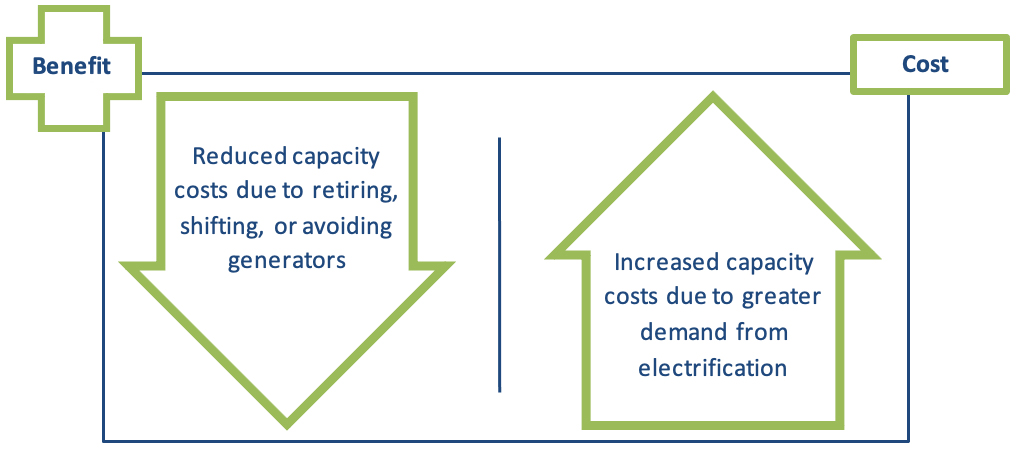 Figure 8. Depiction of benefit/cost factors
3.2.2.b. Methods for Calculating Generation Capacity Impacts
The methods used to determine energy generation values can also be used to determine generation capacity values. This section provides an overview of the common methods, with references to Section 3.1 where relevant. These methods can be used to calculate energy and capacity values separately, or they can be used to calculate energy and capacity values simultaneously. Either way, the estimates of energy and capacity values should be done with consistent inputs and assumptions. For example, the estimates of energy values should assume the same capacity additions that are used in the estimates of capacity values.
Figure 9 below summarizes the most common methods for quantifying or informing generation capacity impacts, each of which is described in detail below. Section 3.2.2.c further summarizes the advantages and disadvantages of each method (see Table 21).
Proxy Unit Method
- Determine capacity saved/created by proposed DER
- Identify most likely proxy unit
- Determine long-term capital and fixed O&M
Peaker Plant Method
- Determine capacity resource on the margin
- Determine per-unit fixed costs of the resource
- Escalate fixed costs over study period
Market Data Method
- Use market auction results to determine capacity prices through recent auction year
- Determine capacity price forecasts for future years by calculating ratio of auction results to net cost of new entry
Power Sector Modeling
- Method 1: Estimate cost of new entry for marginal units by comparing Reference Case forecast to DER Case forecast
- Method 2: Perform capacity market simulation by modeling resource build-out and dispatch to find avoided capacity costs
Public and Proprietary Forecasts
- Use publicly available historical energy cost data as benchmark
- Use publicly available forecasts as inputs
- Obtain proprietary generation capacity impact forecasts to use as inputs, if possible
Figure 9. Common methods for quantifying generation capacity impacts
Option 1: Proxy Unit Method
The proxy unit method for calculating generation capacity impacts is similar to that used for avoided energy generation as described in Section 3.2.1.b. The proxy unit method uses a hypothetical generation unit that serves as a proxy to represent the next planned generating unit that is avoided or built due to the deployment of DERs. The proxy unit’s capital and fixed O&M costs set the avoided capacity cost. This method is one of the more simplistic approaches to calculating avoided generation capacity.
The same three steps used to determine energy generation values can be used to determine generation capacity values.
| Step 1
|
Determine the energy saved or generated by the proposed DER
This can be determined using the proposed DERs’ load impact profiles (see Chapter 11). Ideally, the savings or generation would be developed on an hourly basis to reflect the variation across different time periods.
|
| Step 2
|
Identify the proxy unit that is most likely to be avoided or built due to those DERs
The proxy unit can be identified as the next planned generating unit in a utility’s IRP. In the absence of an IRP, proxies can be based on the most likely resource to be installed next to meet capacity needs. Typically, this is a natural gas combustion turbine (NGCT). However, NGCT’s might no longer represent the marginal capacity resource in some states or regions. For example, to better align with the latest IRP modeling results, California’s 2020 Avoided Cost Calculator recently switched from using a NGCT to a 4-hour storage battery storage resource as the marginal generating unit for determining new-build avoided generation capacity costs (see CPUC 2020).
|
| Step 3
|
Determine the long-term capital and fixed O&M costs of the proxy unit
This is typically the cost of building a new power plant, less the value of the energy generated by that resource. This requires conducting a discounted cash flow analysis that includes initial construction costs, fixed operating costs, and financial data, including carrying costs (see U.S. EPA 2018). The resulting costs are then annualized over the expected life of the proxy unit to yield an annual capacity cost per kW.
The equation for calculating annual avoided capital cost is:
Annualized Costs ($ divided by (kW Year)) *Annual Capacity Savings (kW)=Avoided Capital Costs ($ divided by Year)
|
(See UCS 2020 MN; EPA 2018.)
The primary advantages and disadvantages of this method are essentially the same as those for estimating energy generation values. (See Section 3.2.1.b.)
Key Data Sources for Proxy Unit Method
There are several types of data required for the proxy unit method for estimating generation capacity impacts. (See U.S. EPA 2018.)
- Cost and performance of the proxy unit
- NREL’s Jobs and Economic Development Impact (JEDI) model is a free tool designed to allow users to calculate the economic costs and impacts of constructing and operating power generation assets. The tool provides plant construction costs, as well as fixed and variable operating costs. (See NREL JEDI.)
- U.S. EIA’s Annual Energy Outlook Electricity Market Module Chapter contains cost and performance characteristics of new generating technologies. (See U.S. EIA AEO 2022.)
- Lazard Levelized Cost of Energy Analysis provides capital costs and levelized cost of energy for a variety of generation assets. (See Lazard 2020.)
- Capital cost escalation rates, discount rate, and other relevant financial data
- Handy Whitman Index: A proprietary index that can be used to escalate capital costs. (See Handy Whitman 2022.)
The states of Hawaii and Colorado demonstrate use of the proxy unit method to estimate generation capacity impacts, as shown in Table 13.
Table 13. State examples using the proxy unit method to estimate generation capacity impacts
| State
|
Summary
|
| Hawaii
|
The long-term value of capacity represents the cost of building a new CT or CCGT, less the value of the energy generated by the new resource. The total annualized fixed cost of a new capacity resource is calculated using a pro forma model. (See E3 2014.)
|
| Colorado
|
When the Public Service system showed an incremental capacity need, avoided capacity costs were based on the economic carrying charge (ECC) representation of a generic, combustion turbine’s capital and fixed O&M costs. The resulting $/kw-month were escalated over time at an assumption for inflation and were assigned to distributed solar generation for all 12 months of each year. (See Xcel 2013.)
|
Option 2: Peaker Plant Method
This method calculates generation capacity costs “according to the annualized costs of a pure peaking generation plant” (see Christensen Associates 2014). The peaker plant should represent the resource most commonly used to meet peak demand on the system. This method differs from the proxy unit method in that it is not based on the cost of the next planned generating unit; it assumes that DERs reduce the marginal generation resource.
The peaker plant method involves the three key steps shown in Table 14.
Table 14. Steps to calculate generation capacity impacts using the peaker plant method
| Step 1
|
Determine the capacity resource on the margin within the electric system
|
| Step 2
|
Determine the per-unit fixed costs of that marginal resource
The capacity-related portion of the peaker plant’s fixed costs is assumed to represent the avoided cost of generation capacity. These should not include fuel or O&M savings.
|
| Step 3
|
Escalate the fixed costs over the study period
Use an index such as The Handy-Whitman Index, an annual industry-recognized construction cost index.
|
The primary advantages of this method are its simplicity and its reliance on information that can be obtained from public sources. The primary disadvantages are that it may not accurately represent the timing of the capacity need and the actual type of capacity available to the utility.
Key Data Sources for Peaker Plant Method
The data sources listed above for proxy unit method can also be used for the peaker plant method. Table 15 provides examples of states’ use of the peaker plant method to estimate generation capacity impacts.
Table 15. State examples using the peaker plant method to estimate generation capacity impacts
| State
|
Summary
|
| South Carolina
|
Uses a peaker method to forecast avoided energy and capacity costs from Qualifying Facilities. Duke Energy applies peaker cost assumptions published by U.S. EIA for the cost of the avoided combustion turbine unit used to quantify the projected capacity value. (See SC PSC, Docket Nos. 2019-185-E and DOCKET NO. 2019-186-E.)
|
| Georgia
|
Capacity costs for Qualifying Facilities are based on a Proxy Peaker Methodology. (See GPSC 2021.)
|
Option 3: Market Data Method
In restructured states with wholesale capacity markets, generation capacity impacts can be determined by market prices. There are two key sources of data available in these markets that can be used to calculate generation capacity impacts: capacity market clearing prices, and net cost of new entry (Net CONE).
- Wholesale Capacity Markets: There are three wholesale capacity markets in the United States: ISO‐New England Forward Capacity Market (FCM), New York-ISO Installed Capacity Market (ICAP), and PJM Reliability Pricing Model (RPM). These auctions seek to procure sufficient generation capacity to meet projected load three years in advance.
- Net CONE: An estimate of capacity revenue needed by a new generator in its first year of operation to make it economically viable to build a power plant within a specific market. This value is net of any energy or ancillary services revenues and therefore is a suitable proxy for the value of avoided generation capacity.
While the market data method is a relatively simplistic method and based on publicly available data, the year-to-year variation in market prices can make it difficult to forecast capacity prices over the long term. A recent value of solar study in Washington D.C. provides an example of how capacity auction data can be combined with Net CONE values to increase the accuracy of long-term generation capacity forecasts (see Synapse 2017). This study involved the two key steps shown in Table 16.
Table 16. Steps used to calculate generation capacity impacts using market data and Net CONE values
| Step 1
|
Determine capacity prices for 2019/2020
Used PJM Reliability Pricing Model (RPM) auction results for the PEPCO zone to through the 2019/2020 auction year.
|
| Step 2
|
Forecast capacity prices beyond 2019/2020
Calculated a ratio of RPM auction results to Net CONE to account for observed historical variation in transmission constraints, auction price variability, and difference between PEPCO’s Net CONE compared to the PJM-wide Net CONE.
To calculate the ratio, the study used the most recent five-year Net CONE average (adjusted for inflation) as a forecast for both for PEPCO and PJM-wide Net CONE. The study then calculated the historical ratio of RPM results to Net CONE and multiplied that fraction by the forecasted Net CONE to calculate a forecast of capacity value through 2040.
|
The primary advantages of the market data method are that it is low cost, does not rely on models, and can be conducted with publicly available data. The primary disadvantages include that is may not adequately isolate the interaction of energy prices and capacity prices, it is limited to states served by a wholesale capacity market, and historical wholesale capacity auction clearing prices may not be a good indicator of long-term trends.
Key Data Sources Market Data Method
Wholesale capacity markets websites:
- ISO-NE Forward Capacity Market. (See NE-ISO FCM.).
- PJM Reliability Pricing Model. (See PJM RPM.)
- NY-ISO Installed Capacity Market. (See NY-ISO ICAP.)
Net CONE information:
- PJM: Cost of New Entry Reports. (See PJM CONE.)
- ISO-NE: FCM Parameters Section of the following website includes CONE values. (See NE-ISO FCM.)
- MISO: MISO has published a CONE estimate associated with its current 2018-2019 Planning Resource Auction. (See MISO PRAR.)
For examples of states using the market data method to estimate generation capacity impacts, see Table 17 below.
Table 17. State examples using the market data method to estimate generation capacity impacts
| State
|
Summary
|
| New England States
|
AESC 2021 develops avoided capacity prices for annual commitment periods starting in June 2020. The avoided capacity costs are driven by actual and forecasted clearing prices in ISO-NE FCM. AESC 2021 develops avoided capacity prices from the FCM auction prices using the actual results in auctions for delivery years 2021/22 through 2024/25 and calculating the historical results for the rest of the analysis period. The historical capacity prices are determined by matching the supply and demand curves for Forward Capacity Auction (FCA) 12 through FCA 15. The AESC 2021 forecast prices are based on observations made in recent auctions as well as expected future changes in demand, supply, and market rules. (See AESC 2021.)
|
| Maine
|
For a value of solar study, generation capacity costs were based on ISO‐NE Forward Capacity Market (FCM) clearing prices for the years 2014 to 2018. Due to changes in market rules, forecasts of future prices could not be based on historical results and relied on a simulated forecast based on data published in the 2014 IRP for Connecticut, annualized and adjusted for inflation. Capacity cost forecasts after 10 years were increased by a general escalation rate. (See Clean Power Research 2015.)
|
| New York
|
The NY Department of Public Service (DPS) Staff provide Avoided Generation Capacity Costs (AGCCs) at the bulk system based on forecast of capacity prices for the wholesale market. This data is found in the ICAP Spreadsheet Model filed under Case 14-M-0101. The ICAP Spreadsheet converts “Generator ICAP Prices” to “Avoided CGG at Transmission Level” based on capacity obligations for the wholesale market and provides outputs in $/kW-month. The utilities then convert this into $/MW-year in order to match peak load impacts and calculate avoided generation capacity costs. (See ConEdison 2020.)
|
| New Jersey
|
The NJ Cost Test offers two approaches for calculating avoided generation capacity: (1) revenues earned from the PJM capacity market (RPM) associated with offering and clearing energy efficiency into the RPM; or (2) for customers no monetizing capacity into the RPM, avoided capacity equals the difference in capacity costs for the pre-energy efficiency measure baseline minus load after the energy efficiency. (See NJ BPU 2020.)
|
Option 4: Power Sector Modeling Method
The modeling tools discussed in Section 3.2.1.b can also provide generation capacity values. The two types of models commonly used to develop generation capacity impacts are the capacity expansion model and the production cost model. Figure 10 briefly describes those models.
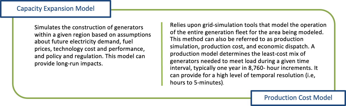 Figure 10. Summary of capacity expansion and production cost models
The choice of model will depend on numerous factors including whether the utility is vertically integrated or part of a capacity market, the needed level of granularity, and the study period.
Depending on these factors there are two methods that are available for estimating avoided capacity. It is important to note that not all capacity expansion and production cost models require the same steps. The methods described below are intended to be generic and may not apply to all models.
Method 1: Estimating Cost of New Entry for marginal units
This method, shown in Table 18, is typically used when deriving avoided generation capacity costs for vertically integrated utilities and can be used if the model does not simulate capacity markets.
Table 18. Steps for estimating Cost of New Entry for marginal units
| Step 1
|
Develop a Reference Case forecast for how load will be met
This forecast should include the customer load expected over the study period but should not include the load impacts of the DERs being evaluated in the BCA (see Section 2.5). This involves entering the following inputs into the model: the projected growth in electricity demand, changes in energy and fuel prices, existing fleet of generating assets, operating characteristics of potential new generating units, and environmental regulations (current and planned). The capacity expansion model uses these inputs to determine a future business-as-usual build-out of the system through an optimization process that chooses the least-cost solution to adding capacity.
|
| Step 2
|
Develop a DER Case forecast
This forecast should include the addition of the DERs being tested for cost-effectiveness over the study period (see Section 2.5). This step involves rerunning the model with the same assumptions except for the addition of DERs over the study period. While capacity expansion models can endogenously select the DER as part of a least-cost portfolio solution, this is not typically done due to data quality issues for DER load impact profiles.
|
| Step 3
|
Calculate the marginal impact
The marginal impact should be calculated by taking the difference in capacity additions between Steps 1 and 2 to calculate the marginal capacity cost per MW based on the annualized capital and fixed costs for all the added resources for the BCA study period.
|
Method 2: Capacity Market Simulation
This method is typically used to develop avoided generation capacity costs for jurisdictions with a capacity market. It is typically run with a production cost model since capacity markets bids and clearing prices rely on accurate energy and ancillary prices that are better determined through a production cost model. Table 19 outlines steps for using this method.
Table 19. Steps for developing avoided generation capacity costs using capacity market simulation
| Step 1
|
Develop a Reference Case forecast for how future load will be met
This involves entering the following inputs into the model: the projected growth in electricity demand, changes in energy and fuel prices, existing fleet of generating assets, operating characteristics of potential new generating units, and environmental regulations (current and planned). The capacity expansion model uses these inputs to determine a future business-as-usual build-out of the system through an optimization process that chooses the least-cost solution to adding capacity. Importantly, this forecast should not include any DERs that will be tested for cost-effectiveness. It may contain other DERs that are not part of the current cost-effectiveness analysis.
|
| Step 2
|
Run the capacity expansion model (and potentially the production cost model)
This process will determine the future resource build-out on the system and simulate dispatch of the resources.
|
The model will output avoided capacity costs in the form of capacity prices (see U.S. EPA 2018).
The primary advantages of the power sector modeling method include its ability to provide granular pricing (hourly and sub-hourly), which can provide a more detailed assessment of how DERs will impact generation. The primary disadvantages include its complexity, required technical expertise, and licensing fees.
Examples of Production Cost and Capacity Expansion Models
See Section 3.2.1.b, Table 8.
Key Data Sources for Capacity Expansion Models
See Section 3.2.1.b.
The states of California and Hawaii demonstrate use of power sector models to analyze generation capacity impacts, shown in Table 20 below.
Table 20. State examples using the power sector model method to estimate generation capacity impacts
| State
|
Summary
|
| California
|
California uses the RESOLVE capacity expansion model and uses a battery storage resource as the proxy for new capacity instead of gas combustion turbine. The capacity avoided cost component was based on the Net CONE of battery storage, using the IRP cost and configuration assumptions and RESOLVE storage build. (See CPUC 2020.)
|
| Hawaii
|
Hawaii has historically used the EnCompass model to calculate annual carrying costs associated with planned capacity additions between 2021 and 2025 on an annual basis. Allocation factors were calculated for both storage and solar resources, and total carrying costs were allocated to on-peak and off-peak hours. Hawaiian Electric plans to use a combination of the RESOLVE & PLEXOS models going forward.
|
Option 5: Publicly Available Generation Capacity Impacts
It is sometimes possible to use generation capacity impacts provided by publicly available sources, instead of the methods described above. The following is a list of publicly available data sources (see U.S. EPA 2018).
Historical Information
Historical energy cost data cannot be directly used as inputs for forward-looking BCAs. Nonetheless, historical energy cost data might be helpful as a starting point for developing forecasts or as a benchmark against which to evaluate forecasts.
- FERC Form 1 provides information for dispatch curve analyses. (See FERC Form 1.)
- SEC 10-Q Filings: Quarterly reports can provide company information on historical financial data and are available from the SEC EDGAR system. (See U.S. SEC EDGAR.)
- Securities and Economic Exchange Commission 10K Filings. The annual filings can provide individual utility historical financial data. (See U.S. SEC EDGAR.)
Forecasts
- Regional Reliability Organizations. For example, NERC has information on required reserve margins. (See NERC website.)
- NREL’s Jobs and Economic Development Impact (JEDI) model. Calculates the economic cost and impacts of constructing power generation assets including plant construction costs and fixed costs. (See NREL Jedi.)
- Avoided Energy Supply Components in New England: 2021 Report provides avoided generation capacity impacts for the six New England States. (See AESC 2021.)
- California Avoided Cost Calculator provides avoided generation capacity impacts for DERs deployed in the state of California. (See CPUC 2021; E3 EE.)
Option 6: Proprietary Generation Capacity Impact Forecasts
Utility filings in resource planning and plant acquisition proceedings often contain long-run avoided costs of power plant capacity. However, utility forecasts are often proprietary. Typically, the only way for non-utility stakeholders to obtain proprietary forecasts is through a docketed case where discovery is permitted.
Accounting for Changes in Reserve Margins
Many electric utilities use a planning reserve margin to ensure that sufficient generation capacity will be available when needed. The reserve margin can vary by utilities and region. They should account for the reliability and operating characteristics of the applicable electricity system. For example, if a utility’s reserve margin is 15 percent and its peak demand is expected to be 100 GW, then it will plan to have 115 GW of capacity installed to ensure that sufficient capacity will be available at the time of peak demand.
DERs can affect the amount of capacity needed to meet the reserve margin by reducing or increasing customer demand. DERs that reduce customer demands, such as energy efficiency, demand response, and distributed generation, will create reserve margin benefits. DERs that increase customer demands, such as building electrification and electric vehicles, will create reserve margin costs.
This planning reserve margin impact can be calculated by multiplying the DER capacity impact (in $ or $/kW) by the planning reserve margin (in %). For example, if a utility has a 15 percent reserve margin, a 10 kW distributed generation resource would actually provide 11.5 kW of capacity benefits because it (a) provides 10 kW of power and (b) reduces the need for 1.5 kW of capacity needed to meet the reserve margin.
3.2.2.c. Choosing a Method to Calculate Generation Capacity Impacts
Table 21 provides a brief description of the advantages and disadvantages of common methods for estimating generation capacity impacts.
Table 21. Advantages and disadvantages of common methods to calculate generation capacity impacts
| Method
|
Description
|
Advantages
|
Disadvantages
|
| Proxy Unit
|
Identifies the next planned generation resource to be built and uses its operational costs as a proxy for avoided energy
|
Simple approach; information available to those outside of utility; does not require detailed data or modeling; inexpensive
|
May produce inaccurate costs; may not apply to DERs with vastly different load impact profiles; does not reflect displacement of baseload units long-term; may miss interactive effects
|
| Peaker Plant
|
Identifies the least-cost capacity option available on the system; capacity-related portion of the unit’s fixed costs assumed to represent the avoided cost of generation capacity
|
Simple approach. Information available to those outside of utility. Does not require detailed data or modeling. Inexpensive.
|
May underestimate costs; may not reflect policy goals of state
|
| Market Data
|
Uses wholesale electricity prices, which reflect the actual costs for operating marginal units in the bids that generators submit
|
Relatively simple approach; captures regional variation. Based on local generation mix; includes transmission congestion
|
Potential to double-count impacts with other avoided costs
|
| Power System Modeling
|
Simulates generation and transmission capacity investment, based on assumptions about future demand, fuel prices, resource cost and performance, and policy and regulation
|
High level of accuracy; captures complex interactions; captures avoided variable costs; can cover longer timeframe up to 40 years; can estimate changes in emissions due to generation mix; can incorporate dispatch characteristics
|
Requires technical expertise and is labor intensive and expensive; lacks transparency due to complexity; choice and accuracy of model impacts are critical to accurate outcomes
|
| Public and Proprietary Forecasts
|
Use publicly available historical energy cost data as benchmark for making forecasts. Use publicly available or proprietary forecasts as inputs.
|
Simple approach; information available to those outside of utility; does not require detailed data or modeling; inexpensive.
|
May not be as granular as desired; may not be as accurate or as up-to-date as other methods; proprietary forecasts might be expensive or unavailable to some stakeholders
|
3.2.2.d. Resources for Calculating Generation Capacity Impacts
Avoided Energy Supply Components Study Group. 2021. (AESC 2021). Avoided Energy Supply Components in New England: 2021 Report. Prepared by Synapse Energy Economics, Resource Insight, Les Demans Consulting, Northside Energy, Sustainable Energy Advantage.
California Public Utilities Commission. 2020. (CPUC 2020). Distributed Energy Resources Avoided Cost Calculator Documentation for the California Public Utilities Commission. Version 1c. Prepared by Energy and Environmental Economics, Inc. June.
Clean Power Research. 2015. Maine Distributed Solar Valuation Study. Prepared for the Maine Public Utilities Commission.
CME Group. n.d. CME Group, Henry Hub. (CME Group website, Henry Hub). “Henry Hub Natural Gas Futures and Options.” cmegroup.com website. www.cmegroup.com/markets/energy/natural-gas/natural-gas.quotes.html.
Crossborder Energy. 2017. The Benefits and Costs of Net Metering Solar Distributed Generation on the System of Entergy Arkansas, Inc. Beach, R. Thomas, and Patrick G. McGuire.
Energy and Environmental Economics, Inc. 2015. (E3 2015). South Carolina Act 236 Cost Shift and Cost of Service Analysis. Prepared on behalf of the South Carolina Office of Regulatory Staff.
Energy and Environmental Economics. n.d. (E3 EE). Energy Efficiency Calculator. EThree.com website. www.ethree.com/public_proceedings/energy-efficiency-calculator/
Federal Energy Regulatory Commission. n.d. (FERC Form 714). “Form No. 714 – Annual Electric Balancing Authority Area and Planning Area Report.” ferc.gov website. www.ferc.gov/industries-data/electric/general-information/electric-industry-forms/form-no-714-annual-electric/data.
Federal Energy Regulatory Commission (FERC). n.d. (FERC Form 1). Form 1 – Electric Utility Annual Report. Ferc.gov website. https://www.ferc.gov/general-information-0/electric-industry-forms/form-1-electric-utility-annual-report
Horizons Energy. n.d. “Horizons Energy National Database.” horizons-energy.com website. http://www.horizons-energy.com/advisory-services/advisory-service-2/.
National Renewable Energy Laboratory. 2014. (NREL 2014 DPV). Methods for Analyzing the Benefits and Costs of Distributed Photovoltaic Generation to the U.S. Electric Utility System. Denholm, P., et al. September.
National Renewable Energy Laboratory. n.d. (NREL ATB). “Electricity Annual Technology Baseline (ATB) Data Download.” atb.nrel.gov website. atb.nrel.gov/electricity/2021/data.
New Jersey Board of Public Utilities. 2020. (NJ BPU 2020). In the Matter of the Clean Energy Act of 2018 – New Jersey Cost Test. Docket Nos. QO19010040 & QO20060389.
National Renewable Energy Laboratory. 2014. (NREL 2014 RPS). Survey of State-Level Cost and Benefit Estimates of Renewable Portfolio Standards. Heeter, J., et. al. May.
North American Electric Reliability Corporation. n.d. (NERC website). Nerc.com website. https://www.nerc.com/pa/RAPA/ra/Pages/default.aspx
Northwest Power and Conservation Council. n.d. (NPCC Forecast). Wholesale Electricity Price Forecast. Nwcouncil.com website. https://www.nwcouncil.org/2021powerplan_wholesale-electricity-price-forecast/
Northwest Power and Conservation Council. n.d. (NPCC Production Cost Simulation). Production Cost Simulation Results. Nwcouncil.com website. https://www.nwcouncil.org/2021powerplan_production-cost-simulation-results/
OpenEI. N.d. (OpenEI State and Local) State and Local Energy Data. OpenEI.com website. https://openei.org/wiki/State_and_Local_Energy_Data
PJM. n.d. (PJM Fuel Data). “Marginal Fuel Type Data.” pjm.com website. www.pjm.com/markets-and-operations/energy/real-time/historical-bid-data/marg-fuel-type-data.aspx.
Regulatory Assistance Project. 2013. (RAP 2013). Recognizing the Full Value of Energy Efficiency. J. Lazar and K. Colburn. https://www.raponline.org/wp-content/uploads/2016/05/rap-lazarcolburn-layercakepaper-2013-sept-09.pdf
Southern Company. 2017. A Framework for Determining the Costs and Benefits of Renewable Resources in Georgia. Revised May 12, 2017. p. 9. https://psc.ga.gov/facts-advanced-search/document/?documentId=167588
Synapse Energy Economics. 2017. (Synapse 2017). Distributed Solar in the District of Columbia: Policy Options, Potential, Value of Solar, and Cost‐Shifting. Prepared for the Office of the People’s Counsel for the District of Columbia.
U.S. Department of Energy. n.d. (U.S. DOE Gateway). “State, Local and Tribal Technical Assistance Gateway.” energy.gov website. www.energy.gov/ta.
U.S. Energy Information Administration. 2020. (U.S. EIA 2020). Capital Cost and Performance Characteristic Estimates for Utility Scale Electric Power Generating Technologies. February.
U.S. Energy Information Administration. 2022. (U.S. EIA AEO 2022). Annual Energy Outlook 2022. https://www.eia.gov/outlooks/aeo/
U.S. Environmental Protection Agency. 2018. (U.S. EPA 2018). Quantifying the Multiple Benefits of Energy Efficiency and Renewable Energy: A Guide for State and Local Governments. www.epa.gov/statelocalenergy/quantifying-multiple-benefits-energy-efficiency-and-renewable-energy-guide-state.
U.S. Environmental Protection Agency. n.d. (U.S. EPA NEEDS). U.S. EPA website. National Electric Energy Data System (NEEDS) v6. www.epa.gov/sites/production/files/2015-08/documents/potential_guide_0.pdf.
U.S. Securities and Exchange Commission. n.d. (U.S. SEC EDGAR). Sec.gov website. https://www.sec.gov/edgar.shtml
White, Kyle. 2019. Direct Testimony and Exhibits. Docket No. EL18-038. “In the Matter of the Compliant of Energy of Utah, LLC and Fall River Solar, LLC Against Black Hills Power Inc. DBA Black Hills Energy for Determination of Avoided Costs.” On Behalf of Black Hills Power, Inc. D/B/A Black Hills Energy.
3.2.3. Renewable and Clean Energy Standard Compliance
3.2.3.a. Definition
In jurisdictions that have adopted a renewable portfolio standard (RPS) or similar regulatory mechanisms like clean energy standards (CES) or clean peak standards (CPS), DERs can impact the cost of compliance. DERs can reduce compliance costs either by reducing the target by virtue of lowering overall electricity demand or increasing the level of qualified renewable or clean energy generation. Alternatively, if a DER has the effect of increasing electricity demand (e.g., electrification) it will require additional renewable purchases and therefore increase the compliance costs of meeting the standard.
3.2.3.b. Methods for Calculating Renewable and Clean Energy Standard Compliance Impacts
Figure 11 summarizes the common methods for quantifying or informing energy generation impacts, each of which is described in detail below. Section 3.2.1.c summarizes the advantages and disadvantages of each method.
Wholesale Electricity Markets Method
- Determine compliance requirements
- Develop REC price forecasts
- Calculate compliance cost per MWh reduction
Vertically Integrated Utilities: Proxy Unit Method
- Choose a proxy unit that represents a typical conventional generator on the system
- Choose a proxy unit that represents a typical conventional generator on the system Compare costs (i.e., fuel, generation capacity, O&M, transmission, ancillary services, emissions) of RPS resources with the levelized cost of the proxy unit
Vertically Integrated Utilities: Modeling Method
- Use dispatch and capacity expansion models to model generation built and dispatched with and without the addition of new renewable energy generation.
Figure 11. Methods for estimating renewable and clean energy standard compliance impacts
Option 1: Wholesale Electricity Markets
For states that have restructured electricity markets, the avoided cost of RPS compliance is typically a function of both the renewable energy certificate (REC) price and load obligation percentage (i.e., the RPS target percentage).
Calculating this impact involves the steps in Table 22.
Table 22. Steps to calculate RES and CES impacts using wholesale electricity market data
| Step 1
|
Review standard to determine compliance requirements
This includes identifying the annual requirements and how they scale over the long term, whether there are different requirements for subcategories or tiers of resources (e.g., new vs. existing resources), and how utilities meet their obligation (e.g., purchasing RECs, building renewable supply, alternative compliance payments).
|
| Step 2
|
Develop REC price forecasts
These should be prepared for each RPS sub-category (if applicable) using forecasts of eligible supply, annual demand targets, and the long-term cost of entry of renewable energy additions. REC prices for “new” resources, where the RPS mandate indicates commercial operation must be achieved after a certain date, are typically based on the cost of new entry for the renewable energy resource. Whereas REC prices for existing resources are typically a function of supply, demand, interaction with other state’s mandate, and alternative compliance payments. (See AESC 2021, pgs. 152-162.)
|
| Step 3
|
Calculate the compliance cost per MWh reduction
This step calculates the RPS compliance cost that DERs avoid or incur through reductions or increases in energy usage. This value can be calculated with the following equation (See AESC 2021):
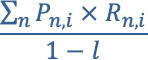
Where:
i = year
n = RPS classes
Pn,i = projected price of RECs for RPS class n in year i,
Rn,i = RPS requirement, expressed as a percentage, for RPS class n in year i,
l = losses from ISO wholesale load accounts to retail meters (%)
|
Table 23 below provides examples of using wholesale electricity market data to estimate Renewable and Clean Energy Standard compliance impacts.
Table 23. State examples of estimating compliance impacts in wholesale electricity markets
| State
|
Summary
|
| New York
|
The compliance cost associated with New York’s Clean Energy Standard (CES) is valued as the resulting $/MWh of a REC from the most recently completed New York State Energy Research and Development Authority RECs solicitation. (See ConEdison 2020.)
|
| Maryland
|
The EmPOWER energy efficiency programs assume that avoided renewable energy requirements result in cost savings that are determined by projecting REC prices. There are different REC prices for Maryland Tier 1 RECs, Maryland Tier 2 RECs, and Maryland Solar RECs. For near-term values, REC prices were based on the futures market for Maryland RECs. For long-term values, Solar REC prices and Tier I REC prices were determined through modeling. Specifically, REC prices were developed by estimating the REC revenue needed to support a 200-MW wind project (Tier 1 REC) and a 10-MW utility-scale solar project (Solar REC). A gap analysis approach was used to determine the REC price necessary to make a wind or solar project economic after accounting for: (1) the capital cost of the project; (2) the cost of capital; (3) O&M expenses; (4) taxes; (5) revenue obtained from the sale of energy and capacity; and (6) the federal investment tax credit (for solar only) (see Exeter Associates 2014, pgs. 19-23).
|
| Pennsylvania
|
The Act 129 energy efficiency programs include the benefit of avoided compliance costs with the state’s Alternative Energy Portfolio Standards Act (AEPS). The Public Utility Commission has access to several subscription-based services that forecast AEC pricing, including Marex Spectron. (See PA PUC 2020.)
|
The primary advantages of this method are that it is a relatively simplistic method and wholesale market data is readily available. The primary disadvantages include that power purchase agreement prices may be proprietary outside of the utility and this approach does not consider the load impact profile of the renewable energy resource and therefore does not consider contribution to on-peak and off-peak periods.
Options 2A and 2B – Vertically Integrated Utilities
The methods for calculating avoided RPS compliance costs for vertically integrated utilities typically involve comparing the cost of procuring the required renewable generation against the cost of procuring the same amount of conventional generation. There are two main methods for this approach (see NREL 2014 DPV):
Option 2A: Proxy Unit Method
This method compares the costs (i.e., fuel, generation capacity, O&M, transmission, ancillary services, emissions) of RPS resources with the levelized cost of a proxy unit that is meant to represent a typical conventional generator on the system. Table 24 below provides examples of states using this method.
The primary advantages of this method are that it is a relatively simplistic method that provides for a long-term outlook by taking the levelized cost over the generation resource life. The primary disadvantages include that it does not account for load impact profiles of renewable resources and does not reflect the fact that RPS requirements could displace more than one type of generation. The proxy unit therefore may not reflect the conventional generation being avoided by the RPS resources, leading to inaccurate avoided costs.
Table 24. State examples using the proxy unit method to estimate compliance impacts
| State
|
Summary
|
| Michigan
|
The PUC is required to determine the cost-effectiveness of the state’s Renewable Energy Standard (RES) as compared to the life-cycle cost of electricity of coal-fired generation. The PUC includes this information where it compares the levelized cost of $133 per MWh for a new coal plant with the combined weighted average levelized renewable energy contract prices for each utility, by RPS technology. In its 2020 report, the PUC noted that “Comparing per unit energy costs of different generation types may not reflect the true value of the resource to the reliability of the electric system as a whole.” (See MPSC 2020, pgs. 16-19.)
|
| Oregon
|
The incremental cost of compliance with the RPS is based on the cost of a combined cycle gas turbine (CCGT), using those filed in the most recent IRP. The proxy type can be changed by the PUC. (See NREL 2014 RPS.)
|
Option 2B: Modeling Method
Similar to the modeling approaches for calculating energy generation impacts, dispatch and capacity expansion models can be used to determine the avoided cost of RPS compliance. This method models generation built and dispatched with and without the addition of new renewable energy generation. Table 25 below shows an example of a state using this method.
The primary advantage of this method is that it produces more accurate results compared to the proxy unit method by producing a comprehensive system view of what would have occurred without the RPS. The primary disadvantages are that it is time intensive, expensive, and lacks transparency due to the complexity of the model.
Table 25. State example using the modeling method to estimate compliance impacts
| State
|
Summary
|
| New Mexico
|
Public Service Company of New Mexico (PNM) calculated RPS costs using a production cost model. PNM models the total system costs with and without each existing and proposed renewable resources to determine the avoided fuel cost for each resource. (See NREL 2014 RPS.)
|
3.2.3.c. Resources for Renewable and Clean Energy Standard Compliance Impacts
Avoided Energy Supply Components Study Group. 2021. (AESC 2021). Avoided Energy Supply Components in New England: 2021 Report. Prepared by Synapse Energy Economics, Resource Insight, Les Demans Consulting, Northside Energy, Sustainable Energy Advantage.
Consolidated Edison Company of New York. 2020. (ConEdison 2020). Electric Benefit Cost Analysis Handbook. Version 3.0
Exeter Associates, Inc. 2014. (Exeter 2014). Avoided Energy Costs in Maryland: Assessment of the Costs Avoided through Energy Efficiency and Conservation Measures in Maryland. Final Report for Power Plant Research Program. Prepared for Maryland Department of Natural Resources.
Michigan Public Service Commission. 2020. (MPSC 2020). Report on the Implementation and Cost-Effectiveness of the P.A. 295 Renewable Energy Standard.
National Renewable Energy Laboratory. 2014. (NREL 2014 DPV). Methods for Analyzing the Benefits and Costs of Distributed Photovoltaic Generation to the U.S. Electric Utility System. Denholm, P., et al. September.
National Renewable Energy Laboratory. 2014. (NREL 2014 RPS). Survey of State-Level Cost and Benefit Estimates of Renewable Portfolio Standards. Heeter, J., et. al. May.
Pennsylvania Public Utility Commission. 2020. (PA PUC 2020). 2021 Total Resource Cost Test Final Order. M-2019-3006868. www.puc.pa.gov/pcdocs/1648126.docx.
3.2.4. Wholesale Market Price Effects
3.2.4.a. Definition
In jurisdictions with competitive wholesale electricity markets, wholesale market prices are a function of the demand of buyers and the marginal costs of suppliers at any given instant. When DERs reduce (or increase) the demand for electricity, they reduce (or increase) the wholesale market prices. This change creates benefits (or costs) for all customers participating in the wholesale market at that time. This effect is sometimes referred to as demand reduction induced price effect (DRIPE).
Figure 12 below shows how a reduction in demand (in this case due to energy efficiency) lowers electricity prices (see Action 2015). Introducing energy efficiency into the market reduces the need to purchase higher cost resources, which will lessen the need for additional generation resource investments. The price delta between the intersection of the supply and the Demand without energy efficiency curves (P1) and the intersection of the Supply and the Demand with energy efficiency curves (P2) is the DRIPE effect. This model holds true provided that the marginal cost of electricity is higher than the average cost.
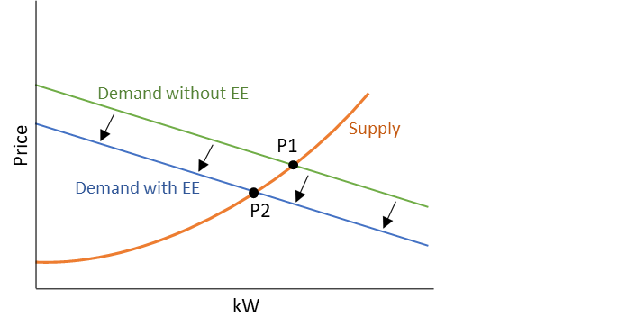 Figure 12. Theoretical effect of DRIPE on the price of electricity
Source: Adapted from DOE 2015, State Approaches to Demand Reduction Induced Price Effects: Examining How Energy Efficiency Can Lower Prices for All, December, page 7.
DERs can impact wholesale market prices either in the form of demand (e.g., distributed solar PV treated as a utility load modifier) or supply (e.g., demand response participation directly in the wholesale market). This impact typically lasts for only a short period before the market adjusts to the new supply/demand balance.
3.2.4.b. Methods for Calculating Wholesale Market Price Effects
The calculation of wholesale market prices effects is dependent on market prices, the size of the market, and the price responsiveness of the market. Figure 13 summarizes two common methods for calculating wholesale market price suppression effects.
Dispatch Curve Analysis
- Determine energy saved or generated by DER
- Develop dispatch curve
- Use dispatch curve to analyze Reference Case
- Use dispatch curve to analyze DER Case
- Take the difference in the wholesale market price between the Reference Case and the DER Case
Combination Analysis
- Calculate the price shift
- Multiply the price shift by total future market demand to create a price-per-demand value
- Adjust the price-per-demand value according to how market operation impacts the total price, timing, and duration of DRIPE
Figure 13. Methods for estimating wholesale market price effects
Option 1: Dispatch Curve Analysis Method
This method involves the steps in Table 26 and can be used for calculating either wholesale energy or capacity market price effects (see EPA 2018, pages 3-34 to 3-36).
Table 26. Steps to calculate wholesale market price effects using the dispatch curve analysis method
| Step 1
|
Determine the energy saved or generated by the proposed DER
This can be determined using the proposed DERs’ load impact profiles (see Chapter 11). Ideally, the savings or generation would be developed on an hourly basis, to reflect the variation across different time periods.
|
| Step 2
|
Develop a dispatch curve
See EPA 2018, Section 3.2.4, beginning on page 3-11.
|
| Step 3
|
Use the dispatch curve to analyze the Reference Case
This is the expected level of electricity demand and resulting costs without the DERs under analysis.
|
| Step 4
|
Use the dispatch curve to analyze the DER Case
This is the expected level of electricity demand and resulting costs with the DERs being analyzed.
|
| Step 5
|
Take the difference in the wholesale market price between the Reference Case and the DER Case
The resulting $/MWh is the wholesale market price effect.
|
Models for Dispatch Curve Analysis Method
This method can be conducted using either spreadsheets, an economic dispatch model like GE MAPS or PROMOD IV, or an energy system model. These tools use data sources such as those provided in Table 27.
Table 27. Key data sources for dispatch curve analysis method
Generator unit data sources: see EPA 2018, pages 3-51 to 3-52.
Option 2: Combination Analysis Method
The AESC 2021 calculates DRIPE for the New England states using a combination of quantitative analyses based on national and New England data instead of modeling projected market conditions. The AESC uses the three-step framework summarized below as the basis to calculate various forms of DRIPE, including energy DRIPE, capacity DRIPE, and cross-DRIPE. The steps, shown in Table 28, become more or less complex depending on the type of DRIPE being calculated. (See AESC 2021, pages 193-230.)
Table 28. Steps to calculate wholesale market price effects using the combination analysis method
| Step 1
|
Calculate the price shift
This is the change in price due to a change in demand. Depending on the availability of data, this can be calculated using a regression from historical data or based on an assumed supply curve. The AESC uses a regression to calculate energy DRIPE and uses the slope of the most recent New England Forward Capacity Auction supply curve and EnCompass model outputs to calculate capacity DRIPE.
|
| Step 2
|
Multiply the price shift by total future market demand
This creates a price-per-demand value. This step allows for the price shift to be applied to any generic change in demand.
Specific to the calculation of capacity DRIPE, the AESC calculates two varieties of capacity DRIPE effects:
- Cleared DRIPE benefits, which are benefits of measures that clear in the ISO-NE Forward Capacity Market (FCM). (See AESC 2021, pgs. 211-212.)
- Uncleared DRIPE benefits, which are benefits of measures that are not submitted into or otherwise do not clear in the ISO-NE FCM. (See AESC 2021, pgs. 213-214.)
|
| Step 3
|
Adjust the price-per-demand value
This step involves estimating the way market operation impacts the total price, timing, and duration of DRIPE.
For example, in calculating energy DRIPE, the AESC reduces the value of DRIPE by the portion of demand that was not already purchased through long-term contracts. This can also have the effect of delaying the realization of DRIPE impacts for several years. The value is further adjusted to reflect the fact that electricity generators will gradually react to the new market price, thereby eroding the price effects from DERs over time.
|
The resulting DRIPE values are provided for each state in intra-zonal terms (including only those benefits associated with load impacts within a zone) and inter-zonal terms (also referred to as rest-of-pool) where benefits accrue outside state borders. Energy DRIPE results are provided in $/kWh and can be applied to DER energy savings or increases in each of the four costing periods (summer on- and off-peak, winter on- and off-peak). Capacity DRIPE results are in $/kW and should be applied to changes in peak energy demand.
Key Data Sources for Combination Analysis Method
- Energy Price data can be obtained from ISOs
- Hourly energy price data and gross load data for ISO-NE. (See ISONE Hourly Data.)
- Sub hourly data for ISO-NE fuel mix. (See ISONE Fuel Mix.)
- Daily data on delivered prices to Algonquin Citygate available from Natural Gas Intel’s “Algonquin Citygate Daily Natural Gas Price Snapchat.” (See NGI 2021.)
Table 29 describes how three states use the combination analysis method to estimate wholesale market price effects.
Table 29. State examples using the combination analysis method<
| State
|
Summary
|
| Washington D.C.
|
Value of solar study used a 2014 study of PJM’s energy DRIPE that determined a DRIPE energy ratio of 1.17, implying that every 1 percent reduction of energy consumption results in a 1.17 percent reduction in price. DRIPE is shared throughout the RTO, therefore the value to D.C. is roughly 1.57 percent of the benefits. The remaining 98.43 percent of the energy DRIPE benefits flow to other PJM ratepayers and represent a societal benefit. Due to generator build and retirement within PJM, the study assumed DRIPE energy benefits dissipate quickly, in a linear manner over a five-year timeframe. (See Synapse 2017)
|
| Maryland
|
Maryland uses a market simulation model (Ventyx) to forecast future energy and capacity values in specific zones located within PJM. The model is run with and without energy efficiency to calculate the change in price. The resulting price is adjusted for each zone, for the state, and to account for decay over time. (See Exeter 2014 pgs. 32-43)
|
| New Jersey
|
The recent New Jersey Cost Test framework calculates energy DRIPE by “regressing historical electric energy prices as a function of load to determine the impact of load on electric energy prices” and calculates capacity DRIPE “using a linear extrapolation of price differentials between auction results and the scenario in which PJM removes 3000 MW of capacity supply from the bottom of the supply curve in MAAC.” (See NJ BPU 2020)
|
3.2.4.c. Resources for Calculating Wholesale Market Price Effects
Avoided Energy Supply Components Study Group. 2021. (AESC 2021). Avoided Energy Supply Components in New England: 2021 Report. Prepared by Synapse Energy Economics, Resource Insight, Les Demans Consulting, Northside Energy, Sustainable Energy Advantage.
Exeter Associates, Inc. 2014. (Exeter 2014). Avoided Energy Costs in Maryland: Assessment of the Costs Avoided through Energy Efficiency and Conservation Measures in Maryland. Final Report for Power Plant Research Program. Prepared for Maryland Department of Natural Resources.
Illinois Power Agency. 2013. (IPA 2013). Annual Report: The Costs and Benefits of Renewable Resource Procurement in Illinois under the Illinois Power Agency and Illinois Public Utilities Acts.
Natural Gas Intel. n.d. (NGI 2021). “Algonquin Citygate Daily Natural as Price Snapshot.” Naturalgasintel.com website. http://www.naturalgasintel.com/data-snapshot/daily-gpi/NEAALGCG/
New England Independent System Operator. 2019. (ISONE Hourly Data). “2019 SMD Hourly.” www.iso-ne.com/static-assets/documents/2019/02/2019_smd_hourly.xlsx
New England Independent System Operator. n.d. (ISONE Fuel Mix). “Dispatch Fuel Mix.” Iso-ne.com website. https://www.iso-ne.com/isoexpress/web/reports/operations/-/tree/gen-fuel-mix
New England Independent System Operator. n.d. (ISONE Load Forecast). “Load Forecast.” iso-ne.com website. https://www.iso-ne.com/system-planning/system-forecasting/load-forecast/
New Jersey Board of Public Utilities. 2020. (NJ BPU 2020). In the Matter of the Clean Energy Act of 2018 – New Jersey Cost Test. Docket Nos. QO19010040 & QO20060389.
Synapse Energy Economics. 2017. (Synapse 2017). Distributed Solar in the District of Columbia: Policy Options, Potential, Value of Solar, and Cost‐Shifting. Prepared for the Office of the People’s Counsel for the District of Columbia.
U.S. Environmental Protection Agency. 2018. (U.S. EPA 2018). Quantifying the Multiple Benefits of Energy Efficiency and Renewable Energy: A Guide for State and Local Governments. www.epa.gov/statelocalenergy/quantifying-multiple-benefits-energy-efficiency-and-renewable-energy-guide-state.
3.2.5. Ancillary Services
3.2.5.a. Definition
Ancillary services are those services required to maintain electric grid stability. They typically include frequency regulation, voltage regulation, spinning reserves, and operating reserves. These services are either traded in wholesale energy markets or self-supplied by utilities.
A DER’s net effect on ancillary services depends on its load impact profile and what the real-time system conditions are at the time of its operation. Some resources may be actively dispatched to provide ancillary services (for instance, storage providing frequency regulation). Alternatively, even if a DER’s operation is not directly in response to a signal to provide ancillary services, it may nevertheless create an impact. For example, during times when load is ramping up quickly and/or generation resources are ramping down quickly, DERs can provide additional operating reserves, fast frequency response, or ramping services. Excess renewable generation is creating the need for new ancillary services such as load build, fast frequency response, shimmy, and shift. As grid architecture likely evolves to achieve clean energy goals, the role of the distribution utility will also need to evolve. This evolution will create DER planning opportunities for additional capacity and ancillary services within distribution resource planning processes.
A DER that reduces energy consumption would create a benefit by avoiding the average ancillary service price, whereas a DER increasing usage would create a cost equal to the average price.
3.2.5.b. Methods for Calculating Ancillary Services Impacts
Figure 14 summarizes two common methods for calculating ancillary services impacts.
Historical Market Data Method
- Historical data from wholesale markets to determine the average price that DERs would receive from participating in ancillary services markets
- Analyze data to determine trends that can be used to project future prices
Production Cost Model Method
- Use model to calculate revenues based upon DER’s ability to participate in various ancillary services markets
- Model selects the optimal dispatch of resources between energy and ancillary services based on a combination of load and availability and capability of DERs
Figure 14. Methods for calculating ancillary services impacts
Option 1: Historical Market Data Method
This method relies on historical data from wholesale markets to determine the average price that DERs would receive from participating in ancillary services markets. The historical data can be analyzed to determine trends than can be used to project prices into the future.
One useful example of this method is Pepco’s BCA for Locational Constraint Solutions (LCS) to calculate the impact of DERs on Regulation and Operating Reserves (See Pepco 2020). This example is described below.
The calculation for regulation revenue is as follows:
Regulation RevenueClass,Year * Installed CapacityClass,Year = Avoided Regulation BenefitYear
Where:
Regulation RevenueClass,Year ($/MW-Year) is PJM’s most recent forward-looking regulation service revenue estimate used to determine the RPM parameters for the technology class of the DERs making up the LCS. For historical or future delivery years, the revenue estimate is adjusted for inflation. If PJM does not calculate a value for regulation revenue for the LCS DERs, then the LCS does not receive this benefit stream.
Installed CapacityClass,Year (MW) is the LCS’s project-specific projected Installed Capacity rating, determined in accordance with the market rules of the PJM RPM.
The calculation for Operating Reserves is as follows:
SR RevenueClass,Year * Installed CapacityClass,Year + NRSRClass,Year * Installed CapacityClass,Year + 30 Minute Reserve RevenueClass,Year * Installed CapacityClass,Year = Avoided Operating Reserve BenefitClass,Year
Where:
SR RevenueClass,Year ($/MW) is PJM’s most recent forward-looking synchronized reserve service revenue estimate used to determine the RPM Base Residual Auction parameters for the technology class of the DERs making up the LCS. This value is normalized to revenues per MW of Installed Capacity for each technology class. For historical or future delivery years, the revenue estimate is adjusted for inflation.
NSR RevenueClass,Year ($/MW) is PJM’s most recent forward-looking non-synchronized reserve service revenue estimate used to determine the RPM Base Residual Auction parameters for the technology class of the DERs making up the LCS. This value is normalized to revenues per MW of Installed Capacity for each technology class. For historical or future delivery years, the revenue estimate is adjusted for inflation.
30 Minute Reserve RevenueClass,Year ($/MW) is PJM’s most recent forward-looking 30-minute reserve service revenue estimate used to determine the RPM Base Residual Auction parameters for the technology class of the DERs making up the LCS. This value is normalized to revenues per MW of Installed Capacity for each resource class. For historical or future delivery years, the revenue estimate is adjusted for inflation.
Installed CapacityClass,Year (MW) is the LCS’s project-specific projected Installed Capacity rating, determined in accordance with the market rules of the PJM RPM.
Key Data Sources for Market Data Method
Ancillary Services Market Data:
Market prices can be obtained from RTOs and ISOs with markets for ancillary services at the locations shown below.
The primary advantage of this method is its simplistic approach that does not involve modeling and is based on publicly available data. The primary disadvantages are that it assumes historical ancillary service prices trends will continue, which may not always be the case as the electricity system changes significantly in the future. This method also relies on historical data that may not be available where no wholesale markets exist. Table 30 describes how two states use this method.
Table 30. State examples using the historical market data method to estimate ancillary services impacts
| State
|
Summary
|
| New York
|
Avoided ancillary service costs are calculated using the two-year historical NYISO market clearing prices. Likewise, if DERs are anticipated to increase ancillary service costs, the additional cost is calculated using the two-year historical NYISO market clearing prices. (See ConEdison 2020.)
|
| New Jersey
|
New Jersey uses a three-year rolling average of historical prices multiplied by the quantity of ancillary services products not purchased. (See NJ BPU 2020.)
|
Option 2: Production Cost Model Method
This method uses a production cost model to estimate the value of future ancillary services. Revenues are calculated based upon the DER’s ability to participate in various ancillary services markets. The model considers the energy and ancillary components for a specific region through characterization of inputs such as fuel costs, electric load, generating unit characteristics, and transmission constraints. The model selects the optimal dispatch of resources between the energy and the ancillary services based on a combination of load and the availability and capability of DERs.
The model user can choose to conduct a more detailed modeling approach by setting a regional or system-wide requirement for ancillary services. This requirement may include, but is not limited to, operating reserves, spinning reserves, and regulation up and down requirements at an hourly or intra hourly level. Similarly, the model user can specify ramp rates, minimum capacity, and response times for various DERs at the resource or unit level to determine the contribution of various resources towards ancillary services.
This method uses a similar set of data sources as what is required for the product cost model method for energy generation as detailed in Section 3.2.1.b.
The primary advantages of this method are that it can more accurately reflect the electricity system in the future and is able to optimize dispatch across both energy and ancillary service requirements simultaneously. This model can be used for different temporal granularities (i.e., hourly, intra hourly). The primary disadvantages are that it is resource intensive and requires the expertise to operate the model. Table 31 describes how two states use this method to estimate ancillary services impacts.
Table 31. State examples using the production cost model method to estimate ancillary services impacts
| State
|
Summary
|
| California
|
Ancillary services impacts were derived from SERVM production simulation that calculated the net market revenues a battery storage unit, assuming optimal dispatch. Prices are extrapolated beyond the model’s output using a compound annual growth rate. (See CPUC 2020, pages 17-18.)
|
| Hawaii
|
The EnCompass model was used in a recent value of DER study to estimate the marginal costs of ancillary services. Ancillary services were modeled as a 30-minute minimum reserve requirement, which represented the resource’s maximum time to ramp up to contribute to reserves. (See Synapse 2021 HI, pg. 8.)
|
3.2.5.c. Resources for Calculating Ancillary Services Impacts
Avoided Energy Supply Components Study Group. 2021. (AESC 2021). Avoided Energy Supply Components in New England: 2021 Report. Prepared by Synapse Energy Economics, Resource Insight, Les Demans Consulting, Northside Energy, Sustainable Energy Advantage.
California Public Utilities Commission. 2020. (CPUC 2020). Distributed Energy Resources Avoided Cost Calculator Documentation for the California Public Utilities Commission. Version 1c. Prepared by Energy and Environmental Economics, Inc. June.
Consolidated Edison Company of New York. 2020. (ConEdison 2020). Electric Benefit Cost Analysis Handbook. Version 3.0.
New Jersey Board of Public Utilities. 2020. (NJ BPU 2020). In the Matter of the Clean Energy Act of 2018 – New Jersey Cost Test. Docket Nos. QO19010040 & QO20060389.
Pepco. 2020. Benefit-to-Cost Analysis Handbook for Locational Constraint Solutions. Docket FC1130.
U.S. Environmental Protection Agency. 2018. (U.S. EPA 2018). Quantifying the Multiple Benefits of Energy Efficiency and Renewable Energy: A Guide for State and Local Governments. www.epa.gov/statelocalenergy/quantifying-multiple-benefits-energy-efficiency-and-renewable-energy-guide-state.
Synapse Energy Economics. 2021. (Synapse 2021 HI). Development of Time-of-Use Rate Options for Hawaii, filed in Advanced Rate Design Track, Docket 2019-0323. Whited, M., S. Liburd, A.S. Hopkins, A. Takasugi, D. Bhandari, R. Fagan. Prepared for Hawaii Division of Consumer Advocacy.
3.2.6. Environmental Compliance Impacts
3.2.6.a. Definition and Overview
There are many environmental requirements that impact the electric utility system. Utilities experience environmental compliance impacts and pass them on to all customers through revenue requirements and rates. In many cases, DERs will help to reduce the costs of environmental requirements by reducing air emissions and other environmental impacts of electricity generation, transmission, and distribution. In some cases, DERs might increase the costs of environmental requirements, for example if they create a net increase in GHG or criteria pollutant emissions.
Sources of Environmental Requirements
Some of the key environmental regulations that impact the electricity industry include:
- Federal regulations such as the Clean Air Act, the Clean Water Act, and the Resource Conservation and Recovery Act.
- Federal, regional, state, or local GHG emission mandates.
- State or local air, land, or water emission constraints.
The most prevalent environmental requirements for the electricity industry can be grouped into the categories shown in Figure 15.
Pollutant cap-and-trade or market-based mechanisms
- These requirements generally impose a cap on total emissions across a regulated category of units, and then allow more flexibility in compliance by allowing allowances for emissions under this cap to be traded between entities. Key to the determining regulatory costs under these programs is how the allowances are allocated to market participants, which can significantly affect cost of compliance. Examples include the federal U.S. Acid Rain Program for sulfur dioxide emissions and Cross-State Air Pollution Rule (see U.S. EPA CMD); the Regional Greenhouse Gas Initiative in the Northeast (see RGGI, n.d.), and the California GHG Cap-and-Trade Program (see CA ARB 2021).
GHG Emission mandates or targets
- GHG mandates or targets are an increasingly common type of environmental compliance costs. These mandates specify emission reductions relative to a benchmark amount (e.g., 1990 emissions) or sometimes place a cap on total emissions (as in cap-and-trade above). They sometimes limit emissions by a single target year (e.g., 2030), or sometimes limit emissions by increasing amounts for several target years (2030, 2040, 2050). Mandates are legally required, while targets are generally not legally binding. An example of a federal GHG target is the U.S. Nationally Determined Contribution, a 2030 emissions target submitted under the Paris Climate Agreement. Emissions mandates may also be expressed in the form of an emissions rate per unit of electricity. Certain regulatory requirements, like new source performance standards under the U.S. Clean Air Act, are based on an evaluation of available emissions reductions technologies, but are ultimate expressed in the form of an emission mandate (see U.S. 2021 NDC).
Pollution control equipment
- Pollution control equipment costs can include capital, fixed O&M, variable O&M, and fuel costs. Pollution control equipment can be installed at the time of construction of the generation facility, or it can be retrofitted after the facility has been in operation. Fuel switching is another strategy for pollution control in existing plants, and that may or may not require capital investment. For example, many coal plants complied with the U.S. Acid Rain Program by switching from high-sulfur to low-sulfur coal, which did not require significant retrofits. Conversely, switching a coal plant to natural gas co-firing will require a higher level of capital investment (see RAP 2013).
Fees and permits
- The federal Clean Air Act requires most generators to obtain construction permits, as well as an operating permit that requires periodic renewal. State air agencies often impose emission fees on electricity generators for criteria air pollutants (see RAP 2013, pages 31-32).
Figure 15. Common environmental requirements with the electricity industry
Relationship to Societal Environmental Impacts
Societal environmental impacts are the impacts on the environment that occur in the absence of environmental requirements or after the environmental requirements have been met. It is important to distinguish between environmental compliance impacts and societal environmental impacts.4
- Environmental compliance impacts are the direct impacts in dollar terms that will be incurred by the utility and passed on to all customers through revenue requirements and customer rates.
- Societal environmental impacts are imposed on society as a whole but do not affect the cost of electricity services.
This distinction, depicted in Figure 16, is important for two reasons. First, environmental compliance impacts are utility system impacts that will be paid by utility customers and therefore should be included in all BCA tests.5 Societal environmental impacts, on the other hand, do not reflect direct costs that will be paid by utility customers and therefore should be included only in a BCA test if that would be consistent with the jurisdiction’s policy goals.
GHG Emissions Impacts
Utility-System Impacts
Addressed in environmental compliance costs (including current and anticipated compliance costs)
Societal Impacts
Externalities not addressed in environmental compliance costs
Figure 16. Distinction between societal and utility-system GHG emissions impacts
Second, environmental compliance impacts will have very different rate and bill impacts than societal environmental impacts. Environmental compliance impacts will affect utility rates and bills, and therefore should be included in rate, bill, and participation analyses. Societal environmental impacts, on the other hand, are not utility system impacts, will not affect rates or bills, and should not be included in rate, bill, and participation analyses.
Example: Assume that a jurisdiction is participating in RGGI, that the estimated price of a RGGI allowance is $12/ton of carbon dioxide, and that there are no other GHG compliance requirements in this jurisdiction. Further assume that the regulators and other stakeholders in this jurisdiction estimate that the total social cost of GHG emissions is $80/ton. In this case, the environmental compliance impact is $12/ton, and the societal environmental impact is $68/ton ($80-$12). (See CPUC 2020, pages 20-23.)
Anticipated Environmental Requirements
BCAs should account for all environmental requirements expected to be in effect over the study period, including those in place but not yet in effect, and those that are not in place but are likely to be in place during the study period.
A BCA should account for all environmental requirements expected to be in effect over the study period (see RAP 2012; RAP 2013, pages 32-37). This should include requirements that are already established by statutes, regulations, orders, or other directives, even if they have not taken effect yet. If a particular requirement is expected to take effect in three years, for example, then the implications of that anticipated requirement should be applied in the third year of the BCA study period and beyond.
Similarly, BCAs should also account for environmental requirements that have not yet been established but are reasonably likely to be established within the study period. Environmental regulations often become more stringent over time (see RAP 2013, page 29) and failure to account for such changes will understate the actual environmental compliance costs.
There will inevitably be some uncertainty about anticipated environmental regulations, just as there is uncertainty about most of the impacts discussed in this MTR handbook. Probability techniques can be used to address this uncertainty, as described below.
Uncertain Environmental Requirements: There may be situations where it is not entirely clear whether environmental requirements will be imposed on the electric utility. For example, a state might establish a GHG target, but the target is not a binding mandate, or the target is applied to the entire economy and not explicitly applied to electric utilities. In these situations, stakeholders and regulators should estimate the most likely timing and magnitude of the targets on electric utilities using the best information available. To completely ignore uncertain GHG targets will understate the costs of compliance with them in the BCA. This could result in implementation of fewer DERs, which could ultimately result in higher costs to comply with the targets once they are applied to the electric utilities. Methods for addressing uncertainty and risk in BCAs are discussed in Chapter 10.
Environmental Compliance Impacts Are Sometimes Included in Other Impacts
Some environmental compliance impacts are routinely included as part of the cost of building and operating generation, transmission, and distribution facilities. These include, for example, costs of installing environmental controls such as scrubbers to remove sulfur dioxide and nitrogen oxides emissions, water protection standards, local permitting requirements, and wildlife protection requirements. (See RAP 2013.)
Similarly, some pollutants, such as nitrogen oxides, sulfur oxides, and GHG emissions, are regulated through a cap-and-trade program in some jurisdictions. In these cases, the environmental compliance impacts might already be included in the energy generation cost and therefore should not be included in this category of impacts in a BCA. (See ConEdison 2020, pages 7-8.)
To the extent that environmental compliance impacts are already included in the cost of the relevant energy resource, they should not be included in this category of impacts in a BCA to avoid double-counting of these costs.
3.2.6.b. Methods for Calculating Environmental Compliance Impacts
Figure 17 summarizes the most common methods for estimating environmental compliance impacts, each of which is described in detail below.
Impacts of Pollutant Cap-and-Trade Mechanisms
- Determine the energy saved or generated (in MWh) by the proposed DER
- Determine the marginal emission rate (in tons/MWh) using public sources or proxy units
- Calculate avoided emissions (in tons) by multiplying DER energy saved or generated by marginal emission rate
- Determine the price of the pollutant (in $/ton) allowance using public sources or independent forecasts
- Calculate cost of compliance (in $) by multiplying avoided emissions by pollutant allowance price
Impacts of GHG Mandates
- GHG Cost Method using marginal abatement costs to calculate the cost of GHG (in $/ton)
- GHG Cost Method using social cost of carbon to estimate cost of GHG (in $/ton); only in cases where GHG mandate represents a societal abatement goal
- Planning Constraints Method: Design Reference and DER Cases to comply with GHG mandates using the lowest cost resources available in each case
Methods for Calculating Other Impacts
- Pollution Control Equipment Costs: Use publicly available information to determine likely costs for different generation facilities
- Fees and Permits Costs:Use publicly available sources for information on fees and permits required for electricity generators
- Anticipated Environmental Requirements: Use same methods as for existing requirements, but apply uncertaintly techniques to accommodate uncertainty about timing or details of requirements
Figure 17. Methods for estimating environmental compliance impacts
Methods for Calculating Impacts of Pollutant Cap-and-Trade Mechanisms
Environmental compliance impacts associated with cap-and-trade mechanisms can be calculated using the steps provided in Table 32. Additional guidance on steps 2 and 4 is provided below the table.
Table 32. Steps to calculate the impacts of pollutant cap-and-trade mechanisms
| Step 1
|
Determine the energy saved or generated (in MWh) by the proposed DER
This can be developed using the proposed DERs’ load impact profiles (see Chapter 11). Ideally, the energy saved or generated would be estimated on an hourly basis, to reflect the variation across different time periods with different marginal emission rates.
|
| Step 2
|
Determine the marginal emission rate (in tons/MWh)
This step is described further below.
|
| Step 3
|
Calculate the change in emissions (in tons)
Multiply the DER energy saved or generated (from Step 1) by the marginal emission rate (from Step 2).
|
| Step 4
|
Determine the price of the pollutant allowance (in $/ton)
This step is described further below.
|
| Step 5
|
Calculate the cost of compliance (in $)
Multiply the avoided emissions (from Step 3) by the pollutant allowance price (from Step 4).
|
Step 2. Determine the Marginal Emission Rate
Marginal emission rates should ideally be based on long-run marginal rates, to capture the full impact over the BCA study period (see Section 2.7.2). They should also be based on the electricity generators in the region where the DER will be located because rates can be very different for different regions. Further, marginal emission rates should ideally be estimated on an hourly basis because they can change significantly as the marginal electricity generator changes throughout the day (see Section 2.8).
Several options are available for determining marginal emission rates. It is important to note that the NREL Cambium model is the only tool listed below that provides long-run marginal emission rates. The U.S. EPA AVERT model and eGRID model only provide short-run marginal emissions rates. Therefore, if models providing short-run marginal emission rates are used, then it will be necessary to use other sources or to develop an independent forecast to determine long-run marginal costs.
- Public sources:
- NREL Cambium model. Cambium is a tool that assembles structured data sets of hourly cost, emission, and operational data for modeled futures of the U.S. electric sector with metrics designed to be useful for long-term decision-making. Cambium was built to expand the metrics reported in NREL’s Standard Scenarios—an annually released set of projections of how the U.S. electric sector could evolve across a suite of different potential futures, looking ahead through 2050. (See NREL Cambium.) Cambium is the only model listed here that provides long-run marginal emission rates.
- U.S. EPA AVERT model. AVERT is an open-access tool offered by the U.S. EPA to estimate the hourly emissions and generation benefits of energy efficiency and renewable energy policies and programs. AVERT allows users to measure displaced emissions of carbon dioxide, sulfur dioxide, nitrogen oxides, particulate matter, ammonia, and volatile organic compounds, as well as avoided generation mitigated by state or multi-state programs. Stakeholders and regulators can also use the tool to identify likely units and regions impacted by different efficiency or renewable energy programs. The tool tracks each fossil unit’s generation, heat input, and emissions. It is able to identify likely changes in regional emissions when units are retired, replaced, or retrofitted with pollution controls. AVERT uses public data reported to the U.S. EPA by power plants in the United States. (See U.S. EPA AVERT.)
- U.S. EPA eGRID model. The Emissions & Generation Resource Integrated Database is a comprehensive source of data from EPA’s Clean Air Markets Division on the environmental characteristics of almost all electric power generated in the United States. The data includes emissions, emission rates, generation, heat input, resource mix, and many other attributes. eGRID is typically used for GHG registries and inventories, carbon footprints, consumer information disclosure, emission inventories and standards, power market changes, and avoided emission estimates. (See U.S. EPA 2021 eGrid.)
- Other tools. See U.S. EPA 2018, pages 4-42 through 4-56, for descriptions and links to a variety of tools to estimate emissions reductions from power plants.
- ISOs. Some ISOs and RTOs publish marginal emission rates for their electricity system. Examples include ISO-NE 2022; NYISO 2021.
- AESC 2021. This report includes marginal emission rates for carbon dioxide and nitrogen oxides for electric generators and for non-electric fuels in New England (see AESC 2021, pages 364-368).
- Proxy units: Proxy power plants can be used to create simplistic estimates of marginal emission rates. For example, in a region where natural gas combined cycle power plants are on the margin most of the time, then the emission rates from these power plants can be a rough approximation of system-wide marginal emission rates (see NREL 2014 DPV). The main advantage of this method is that it is simple to implement. However, the U.S. EPA AVERT model is also relatively simple to use and provides more accurate results.
Step 4. Determine the Price of the Pollutant Allowance
Several options are available for forecasting pollutant allowance prices:
- Public sources:
- Some ISOs and RTOs publish allowance price forecasts (see CPUC 2020, page 21).
- For RGGI price forecasts, see AESC 2021, pages 105-106.
- Independent forecasts: Forecasts of pollutant allowance prices can be made by assuming a simple growth rate applied to current prices (AESC 2021 uses this approach to forecast sulfur dioxide allowance prices, page 110). Alternatively, independent forecasts can be made by comparing the demand and supply for allowances over time and making assumptions about how prices will increase as demand exceeds supply.
Methods for Calculating Impacts of GHG Mandates
Option 1: GHG Cost Method
Environmental compliance impacts associated with GHG mandates can be calculated using the steps provided in Table 35. These are the same steps used to calculate the impacts of pollutant cap-and-trade mechanisms presented above in Table 32, except for Step 4 where the cost of GHG emissions (in $/ton) is applied instead of the pollutant allowance price. The cost of GHG can be developed using a marginal abatement cost (MAC) or a social cost of carbon (SCC) method, described further below.
Table 33. Steps to calculate the impacts of GHG mandates
| Step 1
|
Determine the energy saved or generated (in MWh) by the proposed DER
This can be developed using the proposed DERs’ load impact profiles (see Chapter 11). Ideally, the energy saved or generated would be estimated on an hourly basis, to reflect the variation across different time periods with different marginal emission rates.
|
| Step 2
|
Determine the marginal emission rate (in tons/MWh)
This step is described above as Step 2 for calculating impacts of pollutant cap-and-trade mechanisms.
|
| Step 3
|
Calculate the change in GHG emissions (in tons)
Multiply the DER energy saved or generated (from Step 1) by the marginal emission rate (from Step 2).
|
| Step 4
|
Determine the cost of GHG emissions (in $/ton)
Apply either an MAC or an SCC (where appropriate). This step is described further below.
|
| Step 5
|
Calculate the cost of compliance (in $)
Multiply the avoided emissions (from Step 3) by the pollutant allowance price (from Step 4).
|
Option 1A. Marginal Abatement Cost Method
The cost of curtailing GHG emissions to meet a certain GHG mandate can be estimated by identifying the carbon abatement option that is most likely to be the marginal option for meeting that mandate. The marginal abatement option is determined by ranking all the potential abatement options from lowest to highest cost (in $/ton of GHG abated) and identifying the last, i.e., marginal, abatement option needed to reduce GHG emissions to a particular level specified.
A marginal abatement cost curve is a way to identify the marginal abatement option. An MAC curve rank-orders a set of resources in terms of their cost-effectiveness in abating GHG emissions. These curves compile all the relevant abatement options in a step function format to allow for prioritization of options based on cost-effectiveness.
Section 7.1.2 provides guidance on how to develop an MAC curve, and Figure 34 in that section presents an example MAC curve. Each block in the curve represents a GHG abatement option, which in this case includes different DER options that can reduce GHG emissions from electricity generation. The width of each block indicates the magnitude of emissions that can be abated by that DER (in tons). The height of each block indicates the cost of each option, in net levelized terms (in $/ton).
The net levelized cost is equal to the levelized cost of the abatement option, minus all the levelized benefits of the option except for the GHG benefits. In this way, the curve indicates the GHG abatement cost of each abatement option, beyond all the other costs and benefits of that option. Presenting the net levelized costs in this way allows for straightforward comparison of many different types of abatement options from many different sectors.
For the purposes of estimating GHG compliance costs, the target level of GHG emissions should be set at the specific level of the relevant GHG mandate in the jurisdiction (e.g., reduction of GHGs to 50 percent of 1990 emissions by 2030). For the purposes of estimating societal GHG impacts, the target level of GHG emissions should be set at a level that reflects a societal abatement goal (e.g., net zero GHG emissions by 2050). Guidance on estimating societal GHG impacts is provided in Section 7.1.2.
The advantage of the marginal abatement cost method is that it can be applied without relying upon production cost or capacity expansion models. The disadvantage is that it can be challenging and resource-intensive to develop a marginal abatement cost curve for the jurisdiction of interest.
Option 1B: Social Cost of Carbon Method
The SCC method represents another way to estimate the cost of carbon in terms of $/ton. It uses the “damage-based” approach to estimate this cost, instead of the “abatement-based” approach of the MAC. The SCC is based on the dollar value of the net cost to society from adding a ton of GHG to the atmosphere in a particular year. Costs include the net impacts to agricultural productivity, human health effects, property damage from flood risk and natural disasters, disruption of energy systems, risk of conflict, environmental migration, and the value of impacts to ecosystems (see U.S. IWG 2021).
Starting in 2008, U.S. federal agencies began regularly estimating the SCC, calculated by an interagency working group (IWG) of experts. Since 2016, the IWG has also estimated the social cost of methane and nitrous oxides. The IWG published an updated set of values for all three types of GHGs in 2021 (see U.S. IWG 2021).
The SCC method can be used to estimate the cost of complying with a GHG mandate only in those jurisdictions that have a mandate to achieve a societal abatement goal, e.g., net zero GHG emissions by 2050. Jurisdictions that have a GHG mandate that is less stringent than this societal abatement goal should not use the SCC method. Instead, they should use the MAC method, where the marginal abatement option is based upon the specific GHG abatement goal of the jurisdiction.
Comparison of the Social Cost of Carbon and the Marginal Abatement Cost Methods
Section 7.1.2 provides a comparison of the MAC and SCC methods for estimating either environmental compliance costs or societal GHG impacts. This comparison is summarized in Table 34.
Table 34. Comparison of societal cost of carbon and marginal abatement cost methods
| Method
|
Description
|
Applications
|
Advantages
|
Disadvantages
|
| Social Cost of Carbon
|
Based on future global damage costs from climate change
|
- For determining the total social cost of GHG emissions
- For determining the cost of compliance with GHG mandates that require meeting a societal GHG goal, e.g., net zero emissions by 2050
|
- Values are readily available
- Values are credible because they were developed and vetted by global experts and federal agencies
- Can be applied to emissions from any sector
- Does not require a specific carbon reduction target
|
- Involves considerable uncertainty and debate about future damage costs
- Value is extremely sensitive to the discount rate chosen and complex modeling assumptions
- Can only be used to determine total social cost of GHG emissions
|
| Marginal Abatement Cost
|
Based on cost of technologies and other options that can be used to abate GHG emissions to a desired level in the jurisdiction of interest
|
- For determining the total social cost of GHG emissions, if a societal GHG goal is used, e.g., net zero emissions by 2050
- For determining the cost of complying with specific GHG targets
|
- Well-suited for determining the cost of compliance with GHG targets that are less stringent than a societal GHG goal
- Based on known technologies with known costs relevant to the jurisdiction
- Reveals the actual costs that might need to be incurred to meet GHG target
|
- Requires concrete emission abatement targets
- Values not easily available; estimates are complex and resource-intensive
- Ideally requires analysis for multiple sectors (electric grid, building, transportation, industry)
|
Option 2: Planning Constraints Method
The most accurate approach for estimating the cost of complying with GHG mandates is to use those mandates as constraints in the resource plans that are created to estimate avoided costs. In other words, the Reference Case and the DER Case (and any sensitivities) should be designed to comply with the GHG mandate using the lowest cost resources available in each case. The Reference Case will have to rely upon a set of clean energy options that does not include new DERs, while the DER Case may not need as many other clean energy options because of the GHG emission reductions available from the DERs.
The most accurate approach for estimating the cost of complying with GHG mandates is to use those mandates as constraints in the resource plans that are created to estimate avoided costs.
The difference in costs between the Reference Case and the DER Case will represent the avoided costs of the system, including the avoided costs of achieving the GHG mandates. In other words, the avoided costs of achieving the GHG mandates will not be identified separately from the other avoided costs. If a separate estimate of the avoided costs of the GHG mandate is desired, then one could do a sensitivity analysis comparing a hypothetical Reference Case that does not meet the GHG mandate with the Reference Case that does meet the GHG mandate. The difference in costs between these two cases will indicate the avoided cost of compliance with the mandate, in the absence of the new DERs.
The advantage of this method is that it is the most accurate way to identify the incremental cost of complying with the GHG mandate, because it is based upon a least-cost modeling of all the GHG abatement options. The disadvantage of this method is that it can be labor intensive, especially if production cost or capacity expansion models are used for analyzing the Reference Case and the DER Case.
Methods for Calculating Other Impacts
Methods for Calculating Pollution Control Equipment Costs
For situations where pollution control equipment costs are not accounted for in the other estimates of avoided costs, several sources of publicly available information can be used to determine what these costs are likely to be for different generation facilities (see U.S. EIA 2020; Synapse 2021 RI).
The costs of pollution control equipment should be put in terms of revenue requirements for the purpose of creating inputs to a BCA. For capital costs, this requires amortizing the costs over the book life of the asset, and estimating the annual depreciation, equity, debt, and taxes associated with those costs. Non-capital costs, such as fuel and O&M costs, are typically recovered from customers on a pass-through basis, and therefore the revenue requirements for them will be the same as the annual costs.
Methods for Calculating Fees and Permits Costs
Information on fees and permits required for electricity generators can be obtained from several publicly available sources (see NCAA 2018; NY DEC 2021; RAP 2013, page 32; and U.S. EPA 2021 NPDES).
Methods for Calculating Anticipated Environmental Requirements
In general, anticipated environmental requirements can be estimated with the same methods as existing requirements. The main difference is that there might be some uncertainty about the timing or the details of the requirements. In these cases, uncertainty techniques can be applied to determine the most likely impacts (see RAP 2013, pages 32-33). For example, if the likelihood of the promulgation of a future environmental regulation is 70 percent, then the environmental compliance cost for that regulation can be multiplied by 70 percent.
3.2.6.c. Resources for Calculating Environmental Compliance Impacts
Avoided Energy Supply Components Study Group. 2021. (AESC 2021). Avoided Energy Supply Components in New England: 2021 Report. Prepared by Synapse Energy Economics, Resource Insight, Les Demans Consulting, Northside Energy, Sustainable Energy Advantage.
California Air Resources Board. n.d. (CARB Cap and Trade). Cap and Trade Program website. ww2.arb.ca.gov/our-work/programs/cap-and-trade-program.
California Air Resources Board. n.d. (CARB Cap and Trade). Cap and Trade Program website. ww2.arb.ca.gov/our-work/programs/cap-and-trade-program.
California Public Utilities Commission. 2020. (CPUC 2020). Distributed Energy Resources Avoided Cost Calculator Documentation for the California Public Utilities Commission. Version 1c. Prepared by Energy and Environmental Economics, Inc. June.
Consolidated Edison Company of New York. 2020. (ConEdison 2020). Electric Benefit Cost Analysis Handbook. Version 3.0.
ISO New England. n.d. “Air Emissions.” iso-ne.com website. www.iso-ne.com/about/key-stats/air-emissions/.
Lazard. 2020. Lazard’s Levelized Cost of Energy Report, Version 14.0. October. www.lazard.com/media/451419/lazards-levelized-cost-of-energy-version-140.pdf.
Lawrence Berkeley National Laboratory. 2018. (LBNL 2018 LCOE). The Cost of Saving Electricity Through Energy Efficiency Programs Funded by Utility Customers: 2009–2015. Ian Hoffman, Charles A. Goldman, Sean Murphy, Natalie Mims, Greg Leventis, and Lisa Schwartz. Energy Analysis and Environmental Impacts Division. June.
National Association of Clean Air Agencies. 2018. (NACAA 2018). NACAA Title V Fees Survey: Compilation of Completed Surveys. June.
National Energy Screening Project. 2020. (NSPM 2020). National Standard Practice Manual for Benefit-Cost Analysis of Distributed Energy Resources. https://naseo.org/nesp/nspm/.
National Renewable Energy Laboratory. 2014. (NREL 2014 Survey). A Survey of State-Level Cost and Benefit Estimates of Renewable Portfolio Standards. J. Heeter, et al.
National Renewable Energy Laboratory. 2014. (NREL 2014 RPS). Survey of State-Level Cost and Benefit Estimates of Renewable Portfolio Standards. Heeter, J., et. al. May.
National Renewable Energy Laboratory. n.d. (NREL Cambium). “Cambium.” nrel.gov website. www.nrel.gov/analysis/cambium.html.
Regulatory Assistance Project. 2012. (RAP 2012). Energy Efficiency Cost-Effectiveness Screening: How to Properly Account for ‘Other Program Impacts’ and Environmental Compliance Costs. T. Woolf et al., Synapse Energy Economics. www.synapse-energy.com/sites/default/files/SynapseReport.2012-11.RAP_.EE-Cost-Effectiveness-Screening.12-014.pdf.
Regulatory Assistance Project. 2013. (RAP 2013). Recognizing the Full Value of Energy Efficiency. J. Lazar and K. Colburn. https://www.raponline.org/wp-content/uploads/2016/05/rap-lazarcolburn-layercakepaper-2013-sept-09.pdf
Regional Greenhouse Gas Initiative. n.d. (RGGI, n.d.). Regional Greenhouse Gas Initiative Website. www.rggi.org/.
Smart Electric Power Association. 2021. (SEPA 2021). “Utility Carbon-Reduction Tracker™” sepapower.org website. sepapower.org/utility-transformation-challenge/utility-carbon-reduction-tracker/.
Synapse Energy Economics. 2021. (Synapse 2021 RI). Macroeconomic Impacts of the Rhode Island Community Remote Net Metering Program. Prepared for the Rhode Island Division of Public Utilities and Carriers. March. www.ripuc.ri.gov/generalinfo/Synapse-CRNM-Macroeconomic-Report-2021.pdf.
U.S. Energy Information Administration. 2020. (U.S. EIA 2020). Capital Cost and Performance Characteristic Estimates for Utility Scale Electric Power Generating Technologies. February.
U.S. Energy Information Administration. 2021. (U.S. EIA Levelized Costs 2021). Levelized Costs of New Generation Resources in the Annual Energy Outlook 2021. www.eia.gov/outlooks/aeo/pdf/electricity_generation.pdf.
U.S. Environmental Protection Agency. n.d. (U.S. EPA NPDES). “National Pollutant Discharge Elimination System (NPDES)”. epa.gov website. www.epa.gov/npdes.
U.S. Environmental Protection Agency. n.d. (U.S. EPA Acid Rain Program). “Acid Rain Program.” epa.gov website. www.epa.gov/acidrain/acid-rain-program.
U.S. Environmental Protection Agency. n.d. (U.S. EPA AVERT). “AVoided Emissions and GeneRation Tool (AVERT).” epa.gov website. www.epa.gov/avert.
U.S. Environmental Protection Agency. n.d. (U.S. EPA eGRID). “Emissions and Generation Resources Integrated Database (eGRID).” epa.gov website. www.epa.gov/egrid.
U.S. Environmental Protection Agency. n.d. (U.S. EPA CAMD). “Clean Air Markets.” epa.gov website www.epa.gov/airmarkets.
U.S. Environmental Protection Agency. 2007. (EPA 2007). Guide for Conducting Energy Efficiency Potential Studies, A Resource of the National Action Plan for Energy Efficiency (NAPEE). www.epa.gov/sites/production/files/2015-08/documents/potential_guide_0.pdf.
United States Government. 2021. (U.S. 2021 NDC). The United States of America Nationally Determined Contribution—Reducing Greenhouse Gases in the United States: A 2030 Emissions Target. www4.unfccc.int/sites/ndcstaging/PublishedDocuments/United%20States%20of%20America%20First/United%20States%20NDC%20April%2021%202021%20Final.pdf.