4.1. Introduction
4.1.1. Applications
This section describes the methods and resources that are used to estimate how changes in natural gas use caused by DER programs will affect the cost of supplying gas to end-use customers. Natural gas system impacts are relevant in several BCA applications:
- When gas utilities implement or support DERs that reduce or increase end-use gas consumption, including non-pipe alternatives.
- When electric utilities implement or support DER programs that reduce or increase end-use gas consumption.
- When electric or gas DERs increase or decrease electricity generation and thereby affect marginal gas-fueled power plants on the electricity system. The resulting gas impacts are used as inputs to the energy generation impacts discussed in Section 3.2.1.
- When BCAs are conducted to inform decisions regarding the decarbonization of the gas industry.
The discussion below addresses gas utility system impacts relevant for each of these applications.
4.1.2. Overview of the Gas Utility System
Figure 22 shows different components of the natural gas industry in the United States, from the production wells to the end-use customers. The natural gas industry can be divided into four major segments: (1) production, (2) gathering and processing, (3) transmission and storage, and (4) distribution. Because the industry is not vertically integrated, BCA studies generally focus on the costs that occur after natural gas enters the transmission network and use market prices to capture the costs that occur before that.
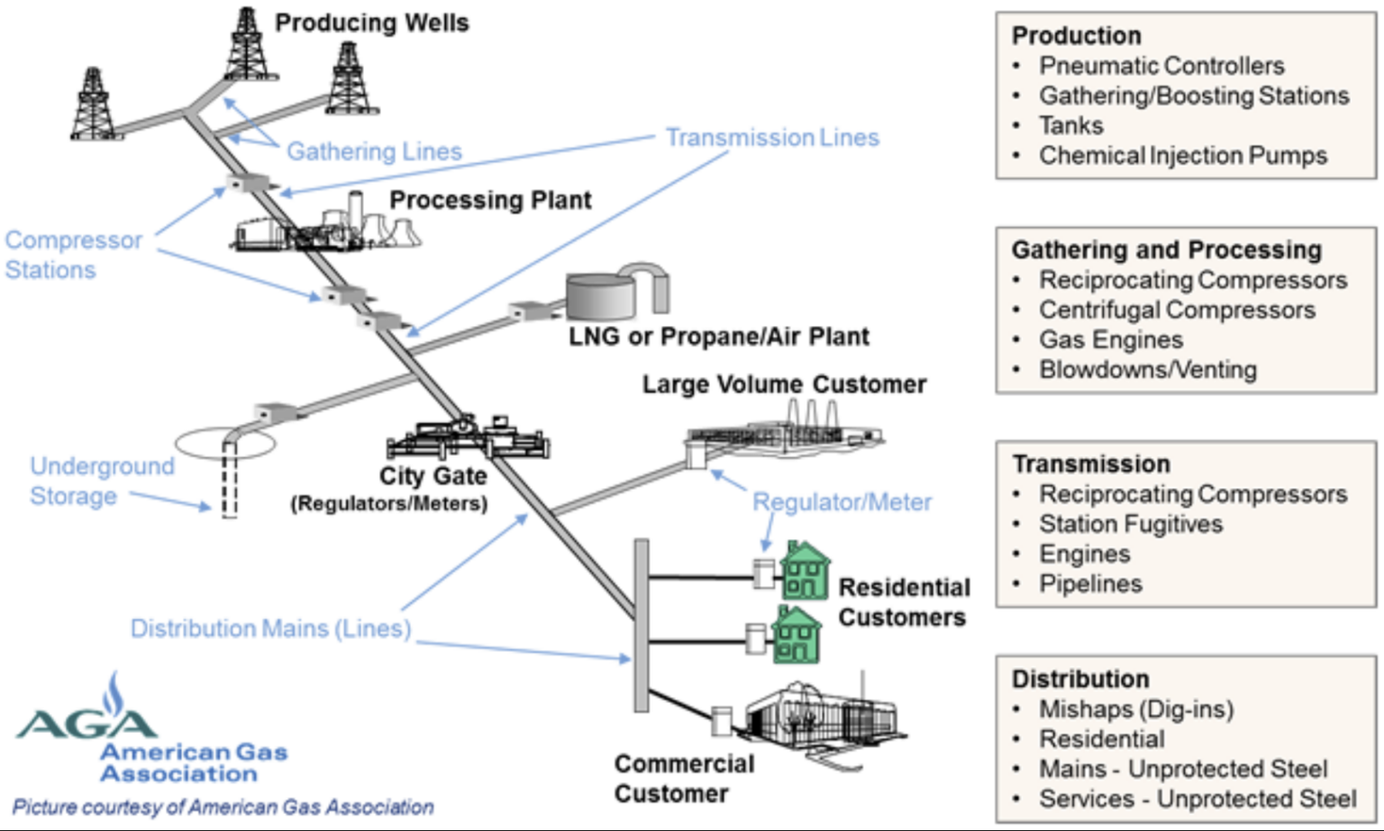 Figure 22. Components of the gas industry in the United States
Source: “Overview of the Oil and Natural Gas Industry,” No date. EPA.gov website. Attribution: American Gas Association
The cost of supplying natural gas to end-use customers generally has three parts:
- The commodity value, which is the market price of natural gas at the location where the gas is purchased.
- The costs associated with the gas transmission, storage, and peaking facilities that deliver gas into the distribution system.
- The distribution system costs to deliver gas to the end-use customer meter.
The first two categories correspond to the gas supply costs that local distribution companies (LDCs) generally recover from customers through the cost of gas rate. The gas transmission, storage, and peaking resource costs in the second category are sometimes referred to as capacity costs. The costs in the third category are included in the LDC’s base distribution rate.9
4.1.3. General Method for Calculating Gas Impacts
The gas utility system impacts of DERs can be estimated by identifying the applicable marginal gas supply resources and multiplying the per-unit cost (usually defined in dollars per MMBtu) by the change in gas use. In general, the cost inputs to this analysis include: (a) commodity costs for each of the costing periods being used for the analysis; (b) transmission, storage, and peaking costs for each of the costing periods; and (c) distribution system costs.
The choice of costing periods will depend on the characteristics of the DER program being analyzed. For example, a gas utility demand response program may lower gas use only during periods of peak gas use, while a gas utility energy efficiency program, such as a water heating program, might reduce gas use throughout the year and have a relatively small impact on peak day requirements.
Several different costing period definitions can be used for this purpose. Examples of costing periods include the following:
- peak day and average day;
- peak day, next nine days, rest of winter period, and rest of year (see AESC 2021, page 40); and
- calendar months.
Monthly costing periods are commonly used when measuring gas cost impacts of natural gas use for electricity generation. Note that monthly costing periods can miss the impacts of high demand days with extreme prices when the electric generator does not hold firm delivered pipeline capacity to the plant.
4.2. Gas Commodity Impacts
4.2.1. Definition
Gas commodity impacts include the costs of purchasing gas at specific locations on the gas system and the variable cost of getting the gas where, and when, it will be used. Natural gas may be purchased:
- within the gas production area;
- at an intermediate market center or hub;
- at the interconnection between a gas transmission system and an LDC (called the “city gate”); or
- at a transmission pipeline meter where gas is delivered directly to an electricity generator or large industrial end-user, bypassing the gas distribution system.
Natural gas is traded as a daily quantity (MMBtu or Mcf per Day). Daily gas deliveries can be “baseload” (a firm, fixed volume of gas which the counterparty commits to purchase each day of a given month for the duration of the contract) or “swing” (a variable daily quantity within a maximum and minimum range). Baseload contracts for the next calendar month are traded toward the end of the previous month. Intra-month “spot” trading is generally done on the last business day before the gas flow day (“day-ahead” purchases).
LDCs typically maintain a portfolio of gas supply resources. These portfolios can include gas purchased at upstream supply points and transported to the city gate on pipeline capacity held by the LDC, and “delivered gas” purchased at the city gate from gas marketers that have access to transportation service on the connecting pipeline.
4.2.2. Methods for Calculating Gas Commodity Impacts
Calculating gas commodity impacts typically starts with forecasts of natural gas prices. In most cases it is only necessary to develop commodity price forecasts for the gas supply resources and purchase locations that are expected to be on the margin during one or more costing periods. The marginal gas supply sources and transportation paths can often be identified from LDC regulatory filings, such as integrated resource plans, rate case testimony, and cost of gas rate applications. These filings typically include information about the supply resources that the LDC plans to acquire to meet projected growth in gas use, or the resources that could be reduced or eliminated if gas use declines.
The impact of a DER on natural gas system commodity costs can also be calculated directly using a dispatch simulation model, such as the Ventyx SENDOUT model. Because these models determine the least-cost dispatch of all available supply resources available to the LDC, this method avoids the need to make assumptions about which resources will be on the margin in each costing period. The impact on commodity costs is calculated by running the dispatch model first with the DER excluded (i.e., a Reference Case), and a second time with the gas use forecast adjusted to include the effect of the DER (i.e., a DER Case). The disadvantage of this approach is that it requires detailed resource descriptions and price forecasts for all of the resources in the LDC supply portfolio.
There are two commonly used methods for developing natural gas price forecasts, shown in Figure 23.
Henry Hub Plus Basis Method
- Use Henry Hub prices as benchmark for forecasting prices at other locations
- Add a “basis” forecast to Henry Hub price to develop price forecast for each location
- Convert price forecasts to costing periods
Gas Market Models Method
- Obtain price forecasts directly from natural gas market models
- Convert price forecasts to costing periods
Figure 23. Summary of methods for calculating gas commodity impacts
Option 1: Henry Hub Plus Basis
Henry Hub prices are often used as the benchmark for forecasting prices at other locations. The price forecast for each location is developed by adding a “basis” forecast to the Henry Hub price.
Henry Hub price forecast
Natural gas future prices are common sources for short-term price forecasts. Natural gas futures prices are not forecasts, per se, but they are widely used as an indicator of market expectations for natural prices at key hubs throughout the United States. Futures prices for gas delivered at Henry Hub are available from public sources (see CME Group, Henry Hub).
Price forecasts can be based on the futures contract settlement prices for a single trading day or, to reduce the effect of day-to-day volatility, on an average of settlement prices over a longer time period. Futures contracts are listed for a period of 12 calendar years, but trading activity drops off after the first two years. Because the lack of trading activity means that the settlement prices for later periods are less meaningful, a common practice is to use the futures prices for the first two or three years of the study period, and then transition to a long-term price forecast from another source.
The most common source of long-term price forecasts for the Henry Hub is U.S. EIA’s Annual Energy Outlook, which provides annual values for the Henry Hub Spot Price for a 30-year period (see U.S. EIA AEO 2022). The main advantage of the AEO forecast is that it is publicly available and well documented. The AEO also includes forecasts for multiple scenarios in addition to the Reference Case. Price forecasts for Henry Hub and other major market centers can also be obtained from other gas market models, some of which are discussed below.
Basis forecasts
There are two alternatives for creating basis forecasts.
First, financial derivatives, such as basis futures and swaps, are used to hedge natural gas prices relative to the Henry Hub price for a number of trading locations. The Intercontinental Exchange provides a platform for trading natural gas basis futures (see AESC 2021, page 28). Forward basis prices are also available from information services such as Natural Gas Intelligence (see NGI 2021) and S&P Global (see S&P Global 2021).
Second, a basis relationship can be calculated by taking the difference between the historical prices for Henry Hub and the historical prices for the trading hub or market area that corresponds to the location where gas will be purchased. Historical basis data should be used carefully because changes in gas market flows and pipeline infrastructure can lead to long-term changes in basis values. For this reason, when using historical basis data for forecasting purposes it would be best to first consider whether the historical basis relationship is likely to remain a reasonable indication of the future relationship.
Option 2: Gas Market Models
Price forecasts for many gas trading locations can be obtained directly from natural gas market models. For example:
- The GPCM® is a widely used tool for “developing market simulations for scenario analysis and forecasts for North American gas flows, price and basis. It is a complete system of interrelated models for simulating gas production, pipeline and storage capacity utilization, deliveries to LDCs, utilities, and industrial consumers, as well as commodity price at points throughout the North American market” (see RBAC GPMC 2021).
- The California PUC uses price forecasts for the two major LDC city gates from the California Energy Commission’s North American Market Gas-trade model (NAMGas) (see CPUC 2020, page 9). The NAMGas model also produces publicly available price forecasts for other gas trading hubs.
- ICF provides a commercially available market forecast for most major market centers using the ICF Gas Markets Model (GMM) (see ICF GMM). The GMM forecasts monthly North American gas production, flows, prices, and basis through 2050.
Converting gas price forecasts to costing periods
Regardless of which option is used, it is also necessary to convert the gas price forecasts to costing periods. Long-term natural gas price forecasts are often calendar-year forecasts that do not correspond to the costing periods being used for the BCA. A common practice is to develop patterns from historical prices or near-term futures prices and apply these multipliers to the annual or monthly forecasts to calculate costing period values. Historical natural gas prices are available for monthly baseload contracts and day-ahead sales for many active trading locations. Price reporting services such as Platts (owned by S&P Global) compile indexes from transaction information obtained from confidential surveys (see Platts 2022).
Variable transportation, storage, and peaking costs
Gas commodity costs also need to include variable transportation, storage, and peaking costs that are incurred after gas is purchased. Methods for estimating these costs are described in Section 4.4.
4.2.3. Method for Calculating the Cost of Gas Used by Electricity Generators
Electricity generators often receive natural gas directly from a gas pipeline operator or from LDCs for unbundled gas transportation service. This is often done through special contracts or tariffs where the distribution cost varies less with changes in gas use than a standard distribution tariff rate. In this situation, the applicable gas supply cost is the commodity price for the gas market area where the generator is located, with typically no capacity or distribution costs added.
4.2.4. Resources for Calculating Gas Commodity Impacts
Avoided Energy Supply Components Study Group. 2021. (AESC 2021). Avoided Energy Supply Components in New England: 2021 Report. Prepared by Synapse Energy Economics, Resource Insight, Les Demans Consulting, Northside Energy, Sustainable Energy Advantage.
California Energy Commission. 2021. (CEC 2021). Natural Gas Burner Tip Prices for California and the Western United States. www.energy.ca.gov/programs-and-topics/topics/energy-assessment/natural-gas-burner-tip-prices-california-and-western.
California Public Utilities Commission. 2020. (CPUC 2020). Distributed Energy Resources Avoided Cost Calculator Documentation for the California Public Utilities Commission. Version 1c. Prepared by Energy and Environmental Economics, Inc. June.
CME Group. n.d. CME Group, Henry Hub. “Henry Hub Natural Gas Futures and Options.” cmegroup.com website. www.cmegroup.com/markets/energy/natural-gas/natural-gas.quotes.html.
ICF International. n.d. (ICF GMM). Gas Markets Model. icf.com website. https://www.icf.com/insights/energy/gas-production-demand
National Gas Intelligence. n.d. (NGI website). NaturalGasIntel.com website. www.naturalgasintel.com.
RBAC, Inc. n.d. (RBAC GPMC). “GPCM® Market Simulator for North American Gas and LNG™” rbac.com website. rbac.com/gpcm-natural-gas-market-model/.
S&P Global. n.d. (S&P Power Forecasts). “Market Intelligence: Power Forecasts.” spglobal.com website. www.spglobal.com/marketintelligence/en/campaigns/power-forecast.
U.S. Energy Information Administration. 2021. (U.S. EIA AEO 2022). Annual Energy Outlook 2021. https://www.eia.gov/outlooks/aeo/
4.3. Gas Wholesale Market Price Effects
4.3.1. Definition
Wholesale market prices are a function of the demand of buyers and the marginal costs of suppliers. When DERs reduce (or increase) the demand for gas, they reduce (or increase) the wholesale market prices, which creates benefits (or costs) for all customers participating in the wholesale market at that time. Even a very small perturbation of the market price can have large impacts when applied across all wholesale customers. This effect is sometimes referred to as demand reduction induced price effect (DRIPE).
4.3.2. Method for Calculating Gas Wholesale Market Price Effects
The wholesale gas market price effects can be calculated using the steps in Table 50.
Table 50. Steps to calculate gas wholesale market price effects
| Step 1 |
Estimate the wholesale gas price elasticity
This is the “price shift,” which represents the change in gas price ($/MMBtu) for a change in gas demand (MMBtu). Aggregated over many data points, this price shift represents the supply curve of a particular DER. Wholesale gas price elasticities are best estimated using an integrated natural gas market forecasting model to assess the impact of a specific change in demand on gas prices at specific market locations. In the absence of such a model, wholesale gas price elasticities can be calculated using a regression analysis, where many historical datapoints are analyzed to establish a relationship between prices and demand. Information for these regression analyses can be obtained from the U.S. EIA (see U.S. EIA AEO 2022).10 |
| Step 2 |
Express the price shift in terms of price-per-demand (in $/MMBtu of demand)
This can then be applied to any generic change in demand. This can be achieved by multiplying the price elasticities by total future market demand. The price-per-demand value can then be multiplied by a DER’s anticipated savings to determine the wholesale market price effect. |
| Step 3 |
Adjust the price-per-demand value to account for market conditions that affect the magnitude of the wholesale market price effect
For gas markets, a portion of non-electric gas consumption is often locked up in short-term contracts and is therefore unresponsive to price changes. Therefore, this portion of gas consumption should be excluded from the calculation. For example, the AESC study assumes that the percentage of non-electric natural gas consumption which is unresponsive to DRIPE varies by year: in year one, 50 percent is assumed unresponsive; in year two, 20 percent is assumed unresponsive; and in year three and all years thereafter 0 percent is assumed unresponsive (see AESC 2021, pages 217 – 218). |
4.3.3. Resources for Calculating Gas Wholesale Market Price Effects
Avoided Energy Supply Components Study Group. 2021. (AESC 2021). Avoided Energy Supply Components in New England: 2021 Report. Prepared by Synapse Energy Economics, Resource Insight, Les Demans Consulting, Northside Energy, Sustainable Energy Advantage.
U.S. Energy Information Administration. 2022. (U.S. EIA AEO 2022). Annual Energy Outlook 2022. https://www.eia.gov/outlooks/aeo/
4.4. Gas Transmission, Storage, and Peaking Impacts
4.4.1. Definition
LDCs typically purchase transmission, storage, and peaking services, or use on-system storage or peaking facilities, to ensure that gas is reliably available when it is needed. Natural gas is stored in depleted gas and oil fields and other underground structures, such as aquifers and salt caverns. Gas is also stored in aboveground tanks as LNG or CNG. Peaking gas supply contracts allow the LDC to call on gas delivered at the city gate during periods of peak gas demand, up to a defined daily quantity and total contract amount. On–system peaking facilities inject vaporized LNG, propane, or compressed natural gas (CNG) directly into the distribution system to supplement the gas supply.
4.4.2. Methods for Calculating Pipeline Transportation Impacts
For most LDCs, the main source of gas capacity costs is the fixed charges for pipeline transportation services that deliver natural gas to the LDC city gate. LDCs typically enter into long-term contracts for pipeline delivery capacity with the option to terminate or continue service at the end of the initial contract term.
Three options for estimating gas transportation costs are described below in Figure 24. Note that if the only gas supply resource is delivered gas purchased at city gate, this step can be omitted. This is often the case for electricity generators that buy gas at pipeline delivery meters that connect directly to the generating plant. Transportation costs are typically included in the wholesale prices that these generators pay for gas fuel and therefore do not need to be determined separately.
Pipeline Tariff Rates Method
- Determine if standard rates are likely to apply (no expansion expected)
- Access current standard rates for interstate pipelines from Informational Postings page on pipeline operator’s website
Incremental Project Rates Method
- Determine if incremental rates are likely to apply (expansion expected)
- Access estimated transportation rates for interstate pipeline expansion projects under development in certificate applications filed with FERC
- Access actual transportation rates for interstate pipeline expansion projects in FERC filings from in-service date
Basis Method
- Use difference between Henry Hub price and retail prices paid by end-use customers as a measure of total transmission and distribution costs for avoided cost analysis
Figure 24. Methods for calculating pipeline transportation impacts
Option 1: Pipeline Tariff Rates
The rates charged by natural gas transmission pipelines in United States are approved by the Federal Energy Regulatory Commission (FERC) and state utility commissions. For interstate pipelines, the tariff rates that are currently in effect can be accessed from the Informational Postings page on the pipeline operator’s website. Transportation charges include the fixed monthly reservation charge, which is paid on the maximum daily quantity that the pipeline operator is obligated to receive and deliver for the customer (or “shipper”) on a given day, and a variable charge based on the pipeline’s variable O&M costs. Pipeline operators also retain a percentage of the gas transported to recover gas used for compressor fuel.
Option 2: Incremental Project Rates
FERC requires natural gas pipeline operators to charge higher “incremental” rates for expansion projects whenever including costs in the standard transportation rate calculation would lead to a subsidization of the project by existing shippers. This means that the transportation rate under a new transportation service agreement can be substantially higher than the rate paid for the same transportation service by shippers holding older contracts.
Choosing which gas transportation rate to use for a BCA will depend on whether gas use is increasing or decreasing, and whether pipeline capacity is expected to be available without new pipeline infrastructure. If gas transmission capacity is expected to expand, so that the DER program will make the expansion larger or smaller (or avoid the need to expand entirely), it is appropriate to use an incremental rate instead of the standard tariff rate. The impact on the avoided capacity cost can be significant for markets with natural gas pipeline capacity constraints. Southern Connecticut Gas Company, for example, estimates that the cost to obtain additional pipeline transportation service to its city gate is more than five times the standard pipeline tariff rate (see Southern Connecticut Gas Company 2020).
Estimated transportation rates for interstate pipeline expansion projects that are in development can be found in the certificate applications filed with FERC. The actual rates for new transportation service agreements are filed around the time that service begins.
Option 3: Basis
The difference between the Henry Hub price and the retail prices paid by end-use customers can be used as a measure of total transmission and distribution costs for avoided cost analysis (see Exeter 2014, page 45). Historical basis data should be used carefully because changes in gas market flows and pipeline infrastructure can lead to long-term changes in basis values.
4.4.3. Method for Calculating Gas Storage Impacts
LDCs purchase natural gas storage services from pipeline operators and independent storage operators. LDCs may also operate on-system storage facilities that connect directly to the distribution system. Gas storage services generally include fixed charges based on the maximum storage capacity quantity and the maximum daily withdrawal quantity, variable charges based on the actual quantities injected and withdrawn, and in-kind charges for storage compressor fuel.
Since most gas storage facilities are regulated by FERC or state utility commissions, these charges can generally be found in the storage operator’s publicly available tariff. Storage facilities operated by LDC involve similar costs, but since these on-system facilities may be physically integrated into the operation of the gas distribution system, these are less likely to be avoidable costs that are affected by a DER program.
There are also significant carrying costs associated with maintaining natural gas storage working gas inventories since the gas in storage must be purchased prior to storage injection, and then held until the gas can be sold after withdrawal.
4.4.4. Methods for Calculating Gas Peaking Impacts
Because LDCs often have more flexibility to adjust their use of gas peaking resources in response to changes in projected end-use customer requirements. Peaking costs are more likely to be avoidable by DERs than, for example, storage costs. Contracts for winter peaking gas delivered at the city gate are often negotiated annually. For on-system peaking facilities, supplies of LNG, propane, and CNG are typically obtained under short-term agreements.
Contracts for peaking resources usually include a fixed reservation charge and a variable charge for the quantity of gas or other fuel that is actually used. However, because the terms of these contracts are often confidential, the actual costs paid by LDCs may not be available from public sources.
4.4.5. Resources for Calculating Gas Capacity Impacts
Avoided Energy Supply Components Study Group. 2021. (AESC 2021). Avoided Energy Supply Components in New England: 2021 Report. Prepared by Synapse Energy Economics, Resource Insight, Les Demans Consulting, Northside Energy, Sustainable Energy Advantage.
California Public Utilities Commission. 2020. (CPUC 2020). Distributed Energy Resources Avoided Cost Calculator Documentation for the California Public Utilities Commission. Version 1c. Prepared by Energy and Environmental Economics, Inc. June.
Exeter Associates, Inc. 2014. (Exeter 2014). Avoided Energy Costs in Maryland: Assessment of the Costs Avoided through Energy Efficiency and Conservation Measures in Maryland. Final Report for Power Plant Research Program. Prepared for Maryland Department of Natural Resources.
Southern Connecticut Gas Company. 2020. Forecast of Natural Gas Demand and Supply, 2021-2025. Filed October 1, 2020 in CT PURA Docket No. 20-10-2, page IV-25.
4.5. Gas Distribution Impacts
4.5.1. Definition
The gas distribution system impacts include the LDC costs to deliver gas from the city gate to retail customers. LDCs operate the gas mains that connect the transmission pipelines and on-system storage and peaking facilities to homes, businesses, and industrial facilities within their service territories. LDCs often provide both bundled service, where the customer buys gas from the LDC, and unbundled service, where the customer buys gas from a marketer and the LDC transports the gas to the customer meter.
LDCs typically recover both fixed and variable costs using volumetric rates. LDCs also retain a percentage of the gas delivered to unbundled customers for gas use and loss.
4.5.2. Methods for Calculating Gas Distribution Impacts
There are several options for calculating the gas distribution system impacts, shown in Figure 25.
LDC Tariffs Method
- Access rates on LDC tariff sheets available from LDC website and/or relevant public utility commission website
Historical Margins Method
- Calculate distribution system costs by taking difference between retail price paid by end-use customers and city gate price
Marginal Cost of Service Study Method
- Use existing marginal cost of service studies to obtain calculations of relationship between plant and O&M expenditures and changes in peak day demand
Engineering Estimates of Avoidable System Upgrade Costs Method
- Use existing engineering studies’ estimates of costs avoided by deferring or avoiding the capital projects that would otherwise be required to meet projected growth in natural gas requirements
Figure 25. Methods for calculating gas distribution impacts
Option 1: LDC Tariffs
LDC rates are a direct measure of the gas distribution system costs paid by end-use customers. These rates can be found on LDC tariff sheets that are often available from the LDC website and/or the relevant public utility commission website.
The gas distribution costs included in LDC rates typically include sunk costs that would not be avoidable by DERs. Therefore, when estimating gas distribution impacts of DERs, LDC rates should be adjusted downward to reflect the portion of rates that can be avoided by DERs.
Option 2: Historical Margins
Distribution system costs can be calculated by taking the difference between the retail price paid by end-use customers and the city gate price. U.S. EIA publishes state-level data, by month, for the city gate price and end-use customer prices by customer class (residential, commercial, and industrial) (see U.S. EIA STEO).
The gas distribution costs included in historical margins can include sunk costs that would not be avoidable by DERs. Therefore, when estimating gas distribution impacts of DERs, historical margins should be adjusted downward to reflect the portion of rates that can be avoided by DERs.
Option 3: Marginal Cost of Service Study
Marginal cost studies use econometric analysis and engineering estimates to calculate the relationship between plant and O&M expenditures and changes in peak day and annual demand. These studies are used to design rates and to set price floors for negotiated-rate contracts. Marginal cost of service studies are commonly included with LDC rate case applications.
Option 4: Engineering Estimates of Avoidable System Upgrade Costs
Engineering studies estimate the costs that are avoided by deferring or avoiding the capital projects that would otherwise be required to meet projected growth in natural gas requirements. The CPUC uses this approach for most end-use customers but uses LDC tariff rates to calculate costs for electric generators (see CPUC 2020, pages 9-10).
4.5.3. Resources for Calculating Gas Distribution Impacts
Avoided Energy Supply Components Study Group. 2021. (AESC Supplemental 2021 Natural Gas). AESC Supplemental Study: Expansion of Natural Gas Benefits. Prepared for AESC Supplemental Study Group. Synapse Energy Economics and Northside Energy.
Avoided Energy Supply Components Study Group. 2021. (AESC 2021). Avoided Energy Supply Components in New England: 2021 Report. Prepared by Synapse Energy Economics, Resource Insight, Les Demans Consulting, Northside Energy, Sustainable Energy Advantage.
California Public Utilities Commission. 2020. (CPUC 2020). Distributed Energy Resources Avoided Cost Calculator Documentation for the California Public Utilities Commission. Version 1c. Prepared by Energy and Environmental Economics, Inc. June.
Energy Institute at Haas. 2021. Who Will Pay for Legacy Utility Costs? L. Davis, C. Hausman. June.
4.6. Targeted Non-Pipe Alternatives
4.6.1. Definition
The methods for calculating transportation capacity impacts related to changes in requirements for gas transmission or distribution facilities apply to the usual situations where DERs have a passive impact on transportation capacity by reducing or increasing natural gas use.
DERs may actively defer pipeline or distribution capacity needs as part of a geographically targeted non-pipe alternative (NPA). This section provides a method for calculating the full set of impacts associated with NPAs. The method is consistent with the method used for NWAs (see Section 3.3.1.c).
4.6.2. Method for Calculating Targeted Non-Pipe Alternatives Impacts
Some DERs can actively defer or avoid investments on specific new pipeline facilities, e.g., through non-pipe alternatives or geographically targeted DERs. In these cases, the pipeline capacity benefits can be determined by calculating the difference in cost between the planned and the deferred installation date of the targeted pipeline investment, using the steps in Table 51 below.
Table 51. Steps to calculate targeted non-pipe alternatives impacts
| Step 1 |
Identify the new transportation facilities that could potentially be avoided by gas DERs
Determine the original date of installation of the new transportation facilities. |
| Step 2 |
Determine the expected cost of the new transportation facilities (in $)
Assume they are installed at the original date of installation (from Step 1). |
| Step 3 |
Determine the amount of gas DER savings (in MMBtu) that will be used to defer the transportation facilities (either transmission or distribution)
This can be done using the proposed DERs’ load impact profiles (see Chapter 11). |
| Step 4 |
Determine the number of years that the new transportation facilities might be deferred by the DER
In some cases, this might be only a year or two; in others it might be indefinitely. |
| Step 5 |
Calculate the expected cost of the new transportation facilities (in $)
Assume they are installed at the later date (from Step 4). |
| Step 6 |
Calculate the difference in costs (in $)
This is the difference between those of the original date (from Step 2) and those of the later date (from Step 4). |
| Step 7 |
Calculate the total avoided transportation cost (in $/MMBtu)
Divide the difference in costs (from Step 5) by the capacity avoided by the DER (from Step 3). |
| Step 8 |
Estimate the annual capital costs (in $/MMBtu-year)
Multiply the total avoided transportation costs (in $/MMBtu) from Step 7 by a real economic carrying charge. The carrying charge should reflect the utility’s cost of capital, income taxes, property taxes, insurance costs, and operation and maintenance expenses. This data is often available as part of utility marginal cost of service studies. |
See AESC Supplemental 2021 Natural Gas, pages 24-34.
4.6.3. Resources for Calculating Non-Pipe Alternative Impacts
Avoided Energy Supply Components Study Group. 2021. (AESC Supplemental 2021 Natural Gas). AESC Supplemental Study: Expansion of Natural Gas Benefits. Prepared for AESC Supplemental Study Group. Synapse Energy Economics and Northside Energy.
Avoided Energy Supply Components Study Group. 2021. (AESC 2021). Avoided Energy Supply Components in New England: 2021 Report. Prepared by Synapse Energy Economics, Resource Insight, Les Demans Consulting, Northside Energy, Sustainable Energy Advantage.
California Public Utilities Commission. 2020. (CPUC 2020). Distributed Energy Resources Avoided Cost Calculator Documentation for the California Public Utilities Commission. Version 1c. Prepared by Energy and Environmental Economics, Inc. June.
Maryland Department of Natural Resources. 2014. (MDNR 2014). Avoided Energy Costs in Maryland: Assessment of the Costs Avoided through Energy Efficiency and Conservation Measures in Maryland. Prepared by Exeter Associates. April.
U.S. Environmental Protection Agency. n.d. (U.S. EPA GWP). “Understanding Global Warming Potentials.” epa.gov website. www.epa.gov/ghgemissions/understanding-global-warming-potentials.
U.S. Environmental Protection Agency. n.d. (U.S. EPA Methane). “Methane Standards.” epa.gov website. www.epa.gov/controlling-air-pollution-oil-and-natural-gas-industry/epa-proposes-new-source-performance.
Zhang et. al. 2020. “Quantifying methane emissions from the largest oil producing basin in the U.S. from space: Methane emissions from the Permian Basin.” Science Advances p. 1-39. https://legacy-assets.eenews.net/open_files/assets/2020/04/23/document_ew_03.pdf.
4.7. Gas System Use and Loss
4.7.1. Definition
Much of the natural gas that flows through gas transmission pipelines and gas distribution systems does not reach the end-use customer. Pipeline operators retain a portion of the gas shipped for compressor fuel, to account for measurement errors, and for actual gas losses.
At the gas distribution level, the difference between the total quantity of gas measured entering the LDC system and the total quantity of gas used delivered to end-use customers or used for gas utility operations is often referred to as lost and unaccounted for (LAUF) gas.
4.7.2. Methods for Calculating Gas System Losses
There are two methods commonly used to estimate losses in the gas system, described in Figure 26.
Tariff Rates Method
- Determine if relevant state tracks LAUF using NRRI survey
- Obtain fuel retainage and LAUF factors from tariff rate postings available on pipeline operator or LDC website
- Determine which categories to include in BCA
Methane Emission Studies Method
- Determine system loss rates using existing studies that analyze gas industry methane emissions to address climate change concerns
Figure 26. Methods for calculating gas system losses
Option 1: Tariff Rates
Natural gas pipeline operators and LDCs typically include fuel retainage and LAUF factors with their tariff rate postings. These factors are generally approved by FERC or state regulators and made available on the pipeline operator or LDC website.
However, delivery loss rates can sometimes be challenging to estimate due to lack of data, differences in costing periods, and more. A 2013 NRRI survey of state regulatory commissions indicates that some states track and report LAUF while many do not. It provides a list of states that report LAUF as well as the LAUF percentages where they are available (see NRRI 2013, pages 91-94).
It is also necessary to determine which categories of use and loss to include in the BCA. For example, by adjusting for gas that the LDC uses for system operations, such as compressors and gas heaters, but excluding losses tied to leakage and inaccurate measurement because these losses are not considered to be directly avoidable.
Option 2: Methane Emission Studies
Gas system loss rates can be determined from studies that analyze gas industry methane emissions to address climate change concerns.11 These studies often look at leakages from the entire gas system, including from wellheads, processing transmission and delivery, and end-use (see Section 7.1.2).
Note that both options described above will typically provide average system losses, rather than marginal losses. Average system losses might be reasonable approximations of marginal losses for many DER types. For some projects, however, additional analysis might be needed to develop marginal losses.
4.7.3. Resources for Gas System Losses
Avoided Energy Supply Components Study Group. 2021. (AESC 2021). Avoided Energy Supply Components in New England: 2021 Report. Prepared by Synapse Energy Economics, Resource Insight, Les Demans Consulting, Northside Energy, Sustainable Energy Advantage.
Alvarez et al. 2018. “Assessment of methane emissions from the U.S. oil and gas supply chain,” Science. 13 Jul 2018. www.science.org/doi/10.1126/science.aar7204.
California Public Utilities Commission. 2020. (CPUC 2020). Distributed Energy Resources Avoided Cost Calculator Documentation for the California Public Utilities Commission. Version 1c. Prepared by Energy and Environmental Economics, Inc. June.
National Regulatory Research Institute. 2013. (NRRI 2013). Lost and Unaccounted-for Gas: Practices of State Utility Commissions. Ken Costello. Report No. 13-06. June.
U.S. Environmental Protection Agency. 2018. (U.S. EPA 2018). Quantifying the Multiple Benefits of Energy Efficiency and Renewable Energy: A Guide for State and Local Governments. www.epa.gov/statelocalenergy/quantifying-multiple-benefits-energy-efficiency-and-renewable-energy-guide-state.
U.S. Environmental Protection Agency. n.d. (U.S. EPA GWP). “Understanding Global Warming Potentials.” epa.gov website. www.epa.gov/ghgemissions/understanding-global-warming-potentials.
U.S. Environmental Protection Agency. n.d. (U.S. EPA Methane). “Methane Standards.” epa.gov website. www.epa.gov/controlling-air-pollution-oil-and-natural-gas-industry/epa-proposes-new-source-performance.
Zhang et. al. 2020. “Quantifying methane emissions from the largest oil producing basin in the U.S. from space: Methane emissions from the Permian Basin.” Science Advances p. 1-39. legacy-assets.eenews.net/open_files/assets/2020/04/23/document_ew_03.pdf.
4.8. Gas Environmental Compliance Impacts
4.8.1. Definition
4.8.1.a. Overview
Gas utilities are required to incur costs for compliance with environmental requirements. These costs are then passed on to all gas customers through revenue requirements and rates. Many such requirements are included in gas fuel and capacity impacts and therefore do not need to be calculated separately.
GHG mandates are a primary environmental requirement that might need to be estimated separately from other fuel impacts. GHG mandates are an increasingly common type of environmental compliance cost in some states. These mandates sometimes require emission reductions relative to a benchmark amount (e.g., 1990 emissions) or sometimes place a cap on total emissions. They sometimes limit emissions by a single target year (e.g., 2030), or sometimes limit emissions by increasing amounts for several target years (2030, 2040, 2050).
The U.S. EPA recently proposed requirements for reducing methane emissions from natural gas transmission and storage facilities (See U.S. EPA website, Methane Standards). These new requirements are likely to impose costs on natural gas that are not accounted for in historical costs or in current forecasts.
4.8.1.b. Relationship to Societal Environmental Impacts
Societal environmental impacts are the impacts on the environment that occur in the absence of environmental requirements or after the environmental requirements have been met. It is important to distinguish between environmental compliance impacts and societal environmental impacts (see Section 3.2.6.).
- Environmental compliance impacts are the direct impacts in dollar terms that will be incurred by the utility and passed on to all customers through revenue requirements and customer rates.
- Societal environmental impacts are imposed on society as a whole but do not affect the cost of gas services.
4.8.1.c. Anticipated Environmental Requirements
BCAs should account for all environmental requirements expected to be in effect over the study period, including those in place but not yet in effect, and those that are not in place but are likely to be in place during the study period.
A BCA should account for all environmental requirements expected to be in effect over the study period (see RAP 2012; RAP 2013, pages 32-37). This should include requirements that are already established by statutes, regulations, orders, or other directives, even if they have not taken effect yet. If a particular requirement is expected to take effect in three years, for example, then the implications of that anticipated requirement should be applied in the third year of the BCA study period and beyond.
Similarly, BCAs should also account for environmental requirements that have not yet been established but are reasonably likely to be established within the study period. Environmental regulations often become more stringent over time (see RAP 2013, page 29) and failure to account for such changes will understate the actual environmental compliance costs.
There may be situations where it is not entirely clear whether environmental requirements will be imposed on the gas utility. For example, a state might establish a GHG target, but the target is not a binding mandate, or the target is applied to the entire economy and not explicitly applied to gas utilities. In these situations, stakeholders and regulators should estimate the most likely timing and magnitude of the targets on the utilities using the best information available. To completely ignore the GHG targets will understate the costs of compliance with them in the BCA. This could result in implementation of fewer DERs, which could ultimately result in higher costs to comply with the targets once they are applied to the utilities.
There will inevitably be some uncertainty about anticipated environmental regulations, just as there is uncertainty about most of the impacts discussed in this MTR handbook. A variety of techniques can be used to address this uncertainty, as described in Chapter 10.
4.8.2. Methods for Calculating Impacts of Compliance with GHG Mandates
Figure 27 summarizes two common methods for estimating impacts of compliance with gas utility GHG mandates.
GHG Cost Method
- MAC method: create marginal abatement cost curve to determine the cost of GHG in terms of $/ton
- SCC method: use social cost of carbon estimates from US IWG to determine the cost of GHG in terms of $/ton
Planning Constraints Method
- Design Reference and DER Cases to comply with GHG mandates using the lowest cost resources available in each case
Figure 27. Methods for estimating impacts of compliance with gas utility GHG mandates
4.8.2.a. GHG Cost Method
Option 1: Marginal Abatement Cost Method
A relatively simple method for estimating the cost of compliance with GHG mandates is to identify the GHG abatement resource that is most likely to be the marginal resource to meet the mandate. The marginal abatement option can be identified by developing a marginal abatement cost curve.
The MAC method for estimating impacts of compliance with electric utility GHG mandates is described in Section 3.2.6.b. The same approach can be used for estimating impacts of compliance with gas utility GHG mandates.
Option 2: Social Cost of Carbon Method
The SCC method represents another way to estimate the cost of carbon in terms of $/ton. It uses the “damage-based” approach to estimate this cost, instead of the “abatement-based” approach of the MAC. The SCC is based on the dollar value of the net cost to society from adding a ton of GHG to the atmosphere in a particular year. Costs include the net impacts to agricultural productivity, human health effects, property damage from flood risk and natural disasters, disruption of energy systems, risk of conflict, environmental migration, and the value of impacts to ecosystems (see U.S. IWG 2021).
The SCC method can be used to estimate the cost of complying with a GHG mandate only in those jurisdictions that have a mandate to achieve a societal abatement goal, e.g., net zero GHG emissions by 2050. Jurisdictions that have a GHG mandate that is less stringent than this societal abatement goal should not use the SCC method. Instead, they should use the MAC method, where the marginal abatement option is based upon the specific GHG abatement goal of the jurisdiction.
The SCC method for estimating impacts of compliance with electric utility GHG mandates is described in Section 3.2.6.b. The same approach can be used for estimating impacts of compliance with gas utility GHG mandates.
Comparison of the Social Cost of Carbon and the Marginal Abatement Cost Methods
Section 7.1.2 provides a comparison of the MAC and SCC methods for estimating either environmental compliance costs or societal GHG impacts. This comparison is summarized in Table 52.
Table 52. Comparison of societal cost of carbon and marginal abatement cost methods
| Method |
Description |
Applications |
Advantages |
Disadvantages |
| Social Cost of Carbon |
Based on future global damage costs from climate change |
- For determining the total social cost of GHG emissions
- For determining the cost of compliance with GHG mandates that require meeting a societal GHG goal, e.g., net zero emissions by 2050
|
- Values are readily available
- Values are credible because they were developed and vetted by global experts and federal agencies
- Can be applied to emissions from any sector
- Does not require a specific carbon reduction target
|
- Involves considerable uncertainty and debate about future damage costs
- Value is extremely sensitive to the discount rate chosen and complex modeling assumptions
- Can only be used to determine total social cost of GHG emissions
|
| Marginal Abatement Cost |
Based on cost of technologies and other options that can be used to abate GHG emissions to a desired level in the jurisdiction of interest |
- For determining the total social cost of GHG emissions, if a societal GHG goal is used, e.g., net zero emissions by 2050
- For determining the cost of complying with specific GHG targets
|
- Well-suited for determining the cost of compliance with GHG targets that are less stringent than a societal GHG goal
- Based on known technologies with known costs relevant to the jurisdiction
- Reveals the actual costs that might need to be incurred to meet GHG target
|
- Requires concrete emission abatement targets
- Values not easily available; estimates are complex and resource-intensive
- Ideally requires analysis for multiple sectors (electric grid, building, transportation, industry)
|
4.8.2.b. Planning Constraints Method
The most accurate approach for estimating the cost of complying with GHG mandates is to use those mandates as a constraint in the resource plans created to estimate avoided costs. In other words, the Reference Case and the DER Case (and any sensitivities) should be designed to comply with the GHG mandate using the lowest cost resources available in each case. The Reference Case will have to rely upon a set of clean energy options that does not include new DERs, while the DER Case may not need as many other clean energy options because of the GHG emission reductions available from the DERs.
The difference in costs between the Reference Case and the DER Case will represent the avoided costs of the system, including the avoided costs of achieving the GHG mandates. In other words, the avoided costs of achieving the GHG mandates will not be identified separately from the other avoided costs. If a separate estimate of the avoided costs of the GHG mandate is desired, then one could do a sensitivity analysis comparing a hypothetical Reference Case that does not meet the GHG mandate with the Reference Case that does meet the GHG mandate. The difference in costs between these two cases will indicate the avoided cost of compliance with the mandate, in the absence of the new DERs.
The advantage of this method is that it is the most accurate way to identify the incremental cost of complying with the GHG mandate, because it is based upon a least-cost modeling of all the GHG abatement options. The disadvantage of this method is that it can be labor intensive.
4.8.3. Resources for Calculating Impacts of Compliance with GHG Mandates
Regulatory Assistance Project. 2012. (RAP 2012). Energy Efficiency Cost-Effectiveness Screening: How to Properly Account for ‘Other Program Impacts’ and Environmental Compliance Costs. T. Woolf et al., Synapse Energy Economics. www.synapse-energy.com/sites/default/files/SynapseReport.2012-11.RAP_.EE-Cost-Effectiveness-Screening.12-014.pdf.
Regulatory Assistance Project. 2013. (RAP 2013). Recognizing the Full Value of Energy Efficiency. J. Lazar and K. Colburn. https://www.raponline.org/wp-content/uploads/2016/05/rap-lazarcolburn-layercakepaper-2013-sept-09.pdf
Smart Electric Power Association. 2021. (SEPA 2021). “Utility Carbon-Reduction Tracker™” sepapower.org website. sepapower.org/utility-transformation-challenge/utility-carbon-reduction-tracker/.
U.S. Environmental Protection Agency. n.d. (U.S. EPA Methane). “Methane Standards.” epa.gov website. www.epa.gov/controlling-air-pollution-oil-and-natural-gas-industry/epa-proposes-new-source-performance.
United States Government. 2021. (U.S. 2021 NDC). The United States of America Nationally Determined Contribution—Reducing Greenhouse Gases in the United States: A 2030 Emissions Target. www4.unfccc.int/sites/ndcstaging/PublishedDocuments/United%20States%20of%20America%20First/United%20States%20NDC%20April%2021%202021%20Final.pdf.
4.9. Gas Utility General Impacts
4.9.1. Financial Incentives Provided by Utility
4.9.1.a. Definition
This impact includes utility financial support provided to DER host customers or other market actors (e.g., retailers, contractors, distributors, manufacturers, integrators, and aggregators) to encourage DER implementation.
Financial incentives may come in various forms, including the following:
- incentives or rebates,
- buy-downs of interest rates for financing a portion of DER costs,
- payments to support trade ally reporting on sales of DERs,
- funding or co-funding of marketing of DER equipment by trade allies, and
- sales bonuses provided to retail or contractor sales staff for selling DER equipment.
4.9.1.b. Methods For Calculating Financial Incentive Impacts
The financial incentives offered to program participants and host customers are typically designed to overcome the market barriers that prevent customers from adopting DERs on their own. They can be based on a variety of factors, including customer surveys (how much is needed to change behavior); payback periods; results from evaluation, measurement, and verification studies; market studies (percent penetration); or rate classifications (e.g., 100-percent incentives for low-income). The financial incentives offered for a DER will depend upon the jurisdiction, the utility, the program design, the DER type, the customer type, and more. Consequently, this information is best obtained by requesting it from the utility, the DER program administrator, or other stakeholders involved in the development of the DER program.
If information is not readily available from the utility or program administrator, these impacts can sometimes be estimated by using data from comparable programs offered by other utilities or program administrators.
4.9.1.c. Resources For Calculating Financial Incentives Impacts
Some energy efficiency and demand response program administrators present information on financial incentives in the prospective energy efficiency plans that they file with regulators to obtain approval of the plans.
4.9.2. Program Administration Costs
4.9.2.a. Definition
Program administration costs are those incurred by the utility related to the planning, design, implementation, and evaluation of a DER program or initiative.
These costs may come in a variety of forms, including costs to support utility outreach to trade allies, technical training, other forms of technical support, marketing, administration, and management of DER programs or portfolios of programs. Administration costs also often include evaluation, measurement, and verification studies to inform either DER program design or retrospective assessment of DER performance.
4.9.2.b. Methods for Calculating Program Administration Costs
DER program administration costs will depend upon the jurisdiction, the program administrator, the program design, the DER type, the customer type, and more. Consequently, this information is best obtained by requesting it from the utility, the DER program administrator, or other stakeholders involved in the development of the DER program.
In some cases, it might be possible to use rough estimates of program administration costs from similar jurisdictions with similar programs. For example, by applying administration costs as a percentage of the total DER program budget to the DER program of interest. This approach, however, should be used with caution because the administration costs can vary depending upon the administrator—even for similar DER programs.
4.9.2.c. Resources For Calculating Program Administration Costs
Most energy efficiency and demand response program administrators present information on program administration costs in the prospective energy efficiency plans that they file with regulators to obtain approval of the plans.
4.9.3. Utility Performance Incentives
4.9.3.a. Definition
In many jurisdictions, utilities are offered shareholder incentives for meeting specific performance metrics related to the success of DER programs. These performance incentives represent a cost associated with the delivery of the DER program.
DER performance incentives can take many forms, including shared savings mechanisms, payments for meeting energy savings targets, payments for meeting capacity savings targets, or combinations of the above. Performance incentives can take the form of rewards, or penalties, or both.
Energy efficiency and demand response programs are frequently supported by utility performance incentives, while it is much less common for such incentives to be applied to other types of DER programs.
4.9.3.b. Methods for Calculating Utility Performance Incentives
Performance incentives are typically set by legislation or regulators and are usually unique to a jurisdiction, state, or utility. They can sometimes be obtained from relevant legislation, regulations, or commission orders. They might also be available from commission dockets used to establish performance incentive mechanisms for a variety of utility services.
Otherwise, this information can be obtained by requesting it from the utility, the DER program administrator, or other stakeholders involved in the development of the utility performance incentive.
4.9.3.c. Resources for Calculating Utility Performance Incentives
Some energy efficiency and demand response program administrators present information on utility performance incentives in the prospective energy efficiency plans that they file with regulators to obtain approval of the plans.
American Council for an Energy Efficient Economy. 2015. (ACEEE 2015 Performance Incentives). Beyond Carrots for Utilities: A National Review of Performance Incentives for Energy Efficiency. Nowak, Baatz, Gilleo, Kushler, Molia, and York. May.
4.9.4. Credit and Collection Costs
4.9.4.a. Definition
This includes costs associated with customers who are deficient on energy bill payments, including notices and support provided to customers in arrears, terminations, disconnections, reconnections, carrying costs associated with arrears, and writing off bad debt.
To the extent that DERs have the effect of lowering a host customer’s energy bill, they might reduce the probability of the customer falling behind or defaulting on bill payment obligations and therefore result in a utility benefit. This may be a particularly important benefit of DER programs targeted to low-income customers.
These are sometimes referred to as utility-perspective non-energy impacts.
4.9.4.b. Methods for Calculating Credit and Collection Costs
These costs tend to depend upon the jurisdiction and the utility being assessed. Some utilities are required to routinely file with regulators information pertaining to their costs associated arrearages, terminations, and other activities related to credit and collection costs (see Narragansett Electric 2021). Many utilities file information on these types of costs as part of their rate cases. In the absence of such publicly available information, these costs can be obtained through information requests to the relevant utility.
Literature reviews can provide some useful information regarding credit and collection costs in other states. (See NEEP 2017 and NMR 2011.)
4.9.4.c. Resources for Calculating Credit and Collection Costs
International Energy Agency. 2014. (IEA 2014). Capturing the Multiple Benefits of Energy Efficiency. www.iea.org/reports/capturing-the-multiple-benefits-of-energy-efficiency.
Narragansett Electric. 2021. Low-Income Monthly Reports. Filed with the Rhode Island Public Utility Commission.
Tetra Tech, NMR Group. 2011. Massachusetts Special and Cross-Sector Studies Area, Residential and Low-Income Non-Energy Impacts (NEI) Evaluation. Prepared for the Massachusetts Program Administrators. ma-eeac.org/wp-content/uploads/Residential-and-Low-Income-Non-Energy-Impacts-Evaluation-1.pdf.
Northeast Energy Efficiency Partnerships. 2017. (NEEP 2017). Non-Energy Impacts Approaches and Values: An Examination of the Northeast, Mid-Atlantic, and Beyond. June. neep.org/sites/default/files/resources/NEI%20Final%20Report%20for%20NH%206.2.17.pdf.
9 LDC rate structures can also include the costs associated with in-franchise peak shaving and storage facilities that are included in some LDC cost of service.
10 Note that there is no one price elasticity for all points on the gas system. The price impact decreases as you move further away from the demand impact. Hence it may be appropriate to use one price impact for the LDC service territory demand but expanding to the state level would require a smaller price impact and expanding to a regional or national impact would require an even smaller impact.
11 There is a distinction between accounting losses and actual methane leakage. Accounting losses are the difference between MMBtu measured at the meter and MMBtu measured at the customer, and thus include differences in meter calibration as well as methane leakages. Almost all of the reported data is based on accounting losses.