Societal impacts should be accounted for in a jurisdiction’s BCA to the extent they are relevant to the jurisdiction’s energy policy goals, consistent with NSPM 2020 guidance.
Electric and gas utility resources can have a variety of impacts that extend beyond the utility system and the host customer. Some or all of these societal impacts should be accounted for in a jurisdiction’s BCA if they are relevant to the jurisdiction’s energy policy goals, consistent with NSPM 2020 guidance. Table 64 summarizes societal impacts commonly associated with DERs.
Greenhouse gases include carbon dioxide, methane, nitrous oxide, and fluorinated gases. GHG emissions are created from a variety of sources, including production, transmission, and distribution of both electricity and natural gas; industrial processes; heating of commercial and residential buildings; and transportation.
Some DER types, such as distributed PV, can reduce GHG emissions by reducing the production and consumption of fossil fuels. Other DER types, such as building electrification and electric vehicles, can increase GHG emissions from electricity generation but reduce GHG emissions by reducing the consumption of other fuels such as gas or gasoline. For these latter DER types, it is important to account for net impact of increased and decreased emissions.
It is important to distinguish between societal GHG impacts and GHG environmental compliance impacts (see Figure 32 and Section 3.2.6.a). Societal GHG emissions represent the emissions that occur after compliance with GHG regulations and requirements. These societal emissions are referred to as “externalities” because the impacts are external to the monetary prices of the goods that create them. The costs of compliance with GHG requirements, on the other hand, are considered “internal” costs because they are passed on to customers in electricity prices.
For example, the cost of compliance with GHG cap-and-trade programs are utility system costs that can be monetized on the basis of the GHG allowance prices (see Section 3.2.6). Any environmental impacts that might result from any remaining GHG emissions are not passed on to utility customers in any way, and therefore should be considered societal impacts.
GHG emissions are often categorized as one of three scopes (See WRI 2015).
Together, all three scopes comprise what is often referred to as life-cycle emissions. It is especially important to calculate impacts for both Scope 1 and Scope 2 GHG emissions, because a decrease in Scope 1 emissions (from on site) is often accompanied by an increase in Scope 2 emissions (from power plants), and vice versa. Scope 3 emissions include the life-cycle emissions associated with manufacturing or disposing of electricity and gas infrastructure, including DERs.
Natural gas or refrigerant leaks could fall into either Scope 1 or Scope 2 depending on the timing, location, and type of leak.
Societal GHG emission impacts can be estimated using the steps shown in Table 65.
Steps 3 and 4 are described in detail below. Steps 1, 2, 5, and 6 are relatively straightforward calculations based on the previous steps.
The magnitude of GHG emissions is often presented in either metric tons (e.g., tonnes) or short tons (e.g., US tons). This handbook uses the term “tons” generically throughout for brevity. In practice it is important to use consistent units throughout any calculation of GHG emissions. Metric tons can be converted into short tons, and vice versa, using the following conversion factor: 1.0 metric tons = 1.10231 short tons.
Building end-use emissions refers to emissions that are produced on site by generating electricity or heating/cooling with fossil fuels, such as natural gas, oil, or propane. Table 66 describes how to calculate the reduction in building end-use GHG emissions from DERs.
Some DERs might affect both a change in consumption at the building end-use (Scope 1) and a change in production at the system level (Scope 2). In these cases, it is important to calculate both impacts.
Table 67 describes how to calculate the reduction in GHG emissions from electric vehicles.
It is important to also calculate the increase in emissions from the purchase of electricity to power the electric vehicle.
The change in GHG emissions from power plants (in tons) caused by DERs can be estimated by multiplying the change in consumption from the DERs (in MWh) by the marginal GHG emissions rates of the electricity system (in tons/MWh).
Marginal emission rates should be based on the electricity generators in the region where the DER will be located because rates can be very different for different regions. Further, marginal emission rates should ideally be determined on an hourly basis because they can change significantly as the marginal electricity generator changes throughout the day (see Section 2.6.) In other words, the hourly change in consumption from the DERS (in MWhs) should be “mapped onto” the hourly marginal emission rates (in tons/MWh).
BCAs should ideally use long-run, as opposed to short-run, marginal emission rates (see Section 2.7.2). Long-run marginal emission rates will capture the changes to emission rates that occur as a result of existing power plants retiring and new electricity resources being added to the system. Marginal emissions rates are expected to change significantly over the coming decades as the electricity system is increasingly powered by renewable generation. In other words, long-run marginal emissions rates may be very different from the short-run emissions of today or those of the next five years. These changes to the electricity system should be accounted for when calculating marginal emission rates over the BCA study period.
There are several sources of marginal GHG emissions rates available to the public, listed below. The U.S. EPA AVERT model and eGRID model provide only short-run marginal emissions rates. If the model used does not estimate long-run marginal emission rates, then it will be necessary to use other sources or to develop an independent forecast to determine those (see AESC 2021).
GHG emissions can result from leaks in the gas and electricity systems. This can include natural gas (methane) leaks associated with the distribution of natural gas and refrigerant (fluorinated gases) leaks in cooling equipment, such as residential, commercial, and industrial refrigerators and heat pumps (see CPUC 2020).16 Methane and fluorinated gases have high global warming potential (GWP), meaning they have a disproportionately high impact on global warming.
Calculating the magnitude of methane leakages from the distribution and consumption of natural gas involves multiplying GHG emissions from gas end-uses by leakage adders. One leakage adder should be used for upstream gas production (gas production, processing, transportation, and delivery) and a separate leakage adder for downstream gas consumption (behind-the-meter usage).17
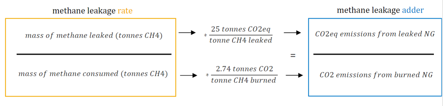 Figure 33. Process for converting methane leakage rate to a leakage adder
Source: CPUC 2020, page 75
Step 4: Calculate the Cost of GHG Emissions in ($/ton)
There are two primary approaches for determining the cost of GHG emissions in $/ton: the social cost of carbon approach and the marginal abatement cost approach. Both approaches yield a value in units of dollars per ton of GHG emissions avoided.
Option 1: Social Cost of Carbon Method
The SCC method (also called the “damage cost” or “damage function” method) is based on the dollar value of the net cost to society from adding an incremental amount of that GHG to the atmosphere in a particular year. Costs include the net impacts to agricultural productivity, human health effects, property damage from flood risk and natural disasters, disruption of energy systems, risk of conflict, environmental migration, and the value of impacts to ecosystems (see U.S. IWG 2021).
Starting in 2008, U.S. federal agencies began regularly estimating the SCC, calculated by an interagency working group (IWG) of experts. Since 2016, the IWG has also estimated the social cost of methane and nitrous oxides. The IWG published an updated set of values for all three types of GHGs in 2021 (see U.S. IWG 2021).
The IWG values are not the only SCC values available. Many estimates have been made by different studies around the world. The IWG SCC values were derived in part by reviewing those other studies and developing values that are appropriate to use by U.S. federal agencies. As such, they are a credible, reasonable source for the purposes of BCAs for DERs.
The value of the SCC is sensitive to many factors, including the choice of model or models to use, damage functions, forecasts of population growth, macroeconomic development, climatological changes, uncertainty analyses, and more.
The value of the SCC is sensitive to many factors, including the choice of model or models to use, damage functions, forecasts of population growth, macroeconomic development, climatological changes, uncertainty analyses, and more (see U.S. IWG 2021, pages 32-35). The models used for this purpose often forecast impacts out to the year 2300, which clearly will involve a great deal of uncertainty. Two factors that are especially important are the perspective of the damages considered (inclusive of damages globally, or only inclusive of damages locally) and the discount rate used to calculate present value dollars (see U.S. IWG 2021; AESC 2021). Thus, while the IWG report presents only a few streams of values for the SCC (one stream for each discount rate) this simple presentation masks the many uncertainties in the analysis and potential range of actual values of damage costs of GHG emissions.
The IWG report presents SCC values for several different discount rates, thus it is necessary to choose a discount rate that is most appropriate for the jurisdiction that the BCA is conducted for. Many experts recommend using a societal discount rate (i.e., 1 to 3 percent) for this purpose (see U.S. IWG 2021; AESC 2021).
Information on the SCC, including information on which climate change impacts are accounted for in the SCC, which states currently use the SCC for planning purposes, and a calculator for calculating the SCC given user-selected parameters, is available on the Institute for Policy Integrity website (see IPI 2021).
Once the SCC value has been determined, the societal GHG impact (in $) can be determined by multiplying the SCC value (in $/ton) by the change in GHG emissions (in tons). Finally, the net societal GHG impact can be determined by subtracting the GHG compliance costs (see Section 3.2.6.b) from the societal GHG impact.
Option 2: Marginal Abatement Cost Method
The societal cost of GHG emissions can be estimating by identifying the carbon abatement option that is most likely to be the marginal option needed to address climate change. The marginal abatement option is determined by ranking all the potential abatement options from lowest to highest cost (in $/ton of GHG abated) and identifying the last, i.e., marginal, abatement option needed to reduce GHG emissions to a level that achieves societal climate change goals (i.e., net zero GHG emissions by 2050).
A marginal abatement cost curve is a way to identify the marginal abatement option. An MAC curve compiles all the relevant abatement options in a step function format to allow for prioritization of options based on cost-effectiveness. Figure 34 presents an example MAC curve. Each block in the curve represents a GHG abatement option, which in this case are different DER options. The width of each block indicates the magnitude of emissions that can be abated by that DER (in tons). The height of each block indicates the cost of each option, using levelized costs (in $/ton).
Levelized costs are used for this purpose because they allow for direct comparison of abatement options that have different operating characteristics and lifetimes. The levelized cost of an energy resource, or a carbon abatement option, represents the full cost of installing and operating the resource over its lifetime, in terms of a single value that applied to each year of the lifetime results in a cumulative present value that is the same as the cumulative present value of the actual stream of annual costs.
Levelized Costs: Levelized costs for electricity generation resources are commonly referred to as the levelized cost of electricity (LCOE) (see EIA 2019). Levelized costs for efficiency resources are commonly referred to as levelized cost of saved energy (LCSE) (see LBNL 2018 LCOE). This handbook uses the term “levelized cost of energy” to refer to both LCOE and LCSE interchangeably.
Publicly available sources. Levelized costs of electricity resources are available from several public sources, including (see Lazard 2021; LBNL 2018 LCOE; U.S. EIA 2021).
Independent estimates. Levelized costs can be calculated for specific resources using the following formulas:
LCOE = (capital recovery factor) * (resource lifetime costs) / (annual generation, in kWh)
LCSE = (capital recovery factor) * (resource lifetime costs) / (annual electricity savings, in kWh)
Capital recover factor = [r*(1+r)^n] / [(1+r)^n-1]
r = the discount rate
MAC curves present the cost of each GHG abatement option in net levelized costs. The net levelized cost is equal to the levelized cost of the abatement option, minus all the levelized benefits of the option, except for the GHG benefits. In this way, MAC curves indicate the GHG abatement cost of each abatement option, beyond all the other costs and benefits of that option (see NSPM 2020, Section 15.5.3).
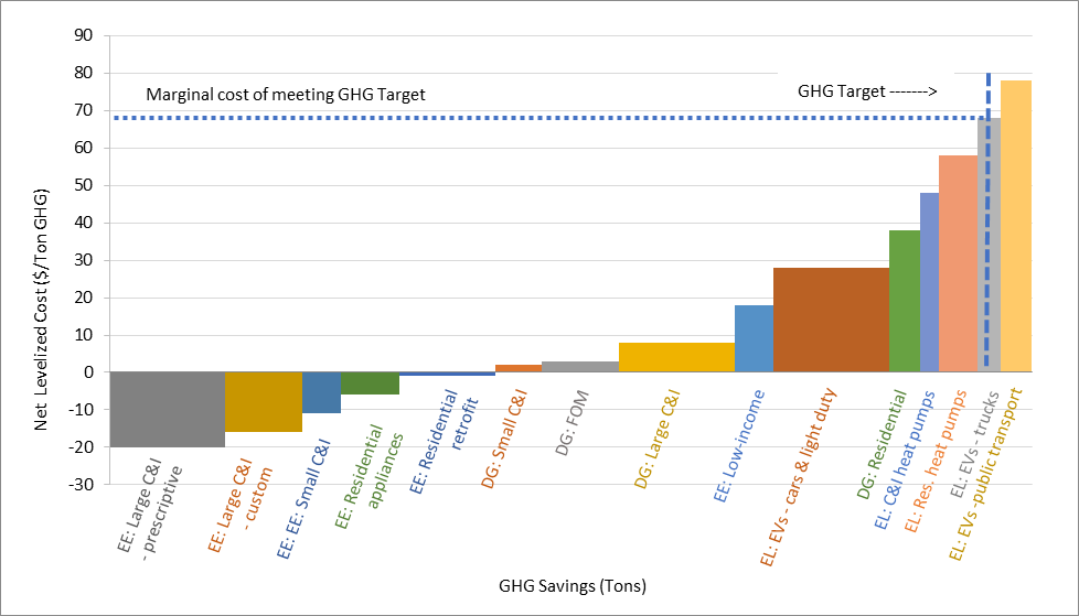 Figure 34. Example marginal abatement cost curve for DERs
Source: Adapted from NSPM 2020, page 13-6, Figure 13-2. The DERs and cost-effectiveness results presented in this figure are purely illustrative and not based on specific DERs in a specific jurisdiction. Actual cost-effectiveness results could be significantly different from those presented here. In addition, actual results will differ depending upon the cost-effectiveness test used.
An abatement option with a net levelized cost below zero is cost-effective without considering the GHG benefits. For those abatement options with a net levelized cost above zero, the cost shown represents only the cost of abating GHG emissions. Presenting the net levelized costs in this way allows for straightforward comparison of many different types of abatement options from many different sectors.
MAC curves are especially useful for calculating the cost of complying with GHG mandates and requirements (see Section 3.2.6.b) because they can be tailored to the specific GHG mandates and requirements of the relevant jurisdiction. They can also be used for calculating societal GHG impacts.
If the marginal abatement cost approach is used to develop the societal impacts of GHGs, then the GHG target should represent a societal abatement goal, e.g., net zero GHG emissions by 2050. If the GHG abatement options used to develop the MAC curve are not sufficient to achieve this societal goal, then the curve will not reveal the full cost necessary to meet that goal.
If the marginal abatement cost approach is used to develop the societal impacts of GHGs, then the GHG target should represent a societal abatement goal, e.g., net zero GHG emissions by 2050.
The MAC can be developed for a given year using a selected carbon dioxide reduction amount. The MAC can be calculated differently based on the region of interest, e.g., global, national, regional, state, local. The MAC can also be calculated differently for the sector of interest, e.g., electric, gas, transportation, industry, others. Ideally, the MAC would include all sectors of the economy to provide a more complete picture of how a jurisdiction might be able to reduce GHGs. For example, if the MAC is being used as a GHG cost for both Scope 1 and 2 emissions, then both Scope 1 and Scope 2 abatement technologies should be included in the curve.
One of the most prominent MAC curves is the McKinsey curve, which considers costs and investments on a global scale (see McKinsey n.d.). Other attempts at making a MAC curve aim to include the impact of behavioral change (see Gillingham and Stock 2018) and using energy optimization models and systems-level analysis (see EDF 2021). New England’s AESC calculates a global and regional marginal abatement cost of carbon. At the regional level, AESC calculates an electric-sector-specific value as well as a value for all sectors (see AESC 2021).
MAC curves can be created using the steps in Table 69 below.
Table 69. Steps to calculate GHG emissions costs using a marginal abatement cost curve
| Step 1 |
Put each DER cost into levelized terms
These can be obtained from publicly available sources or by using formulas to calculate levelized costs using jurisdiction-specific information (see Section 3.2.6.b). This will provide costs in terms of levelized $/MWh. |
| Step 2 |
Put each DER benefit into levelized terms
These are calculated the same as the costs. In this case, public sources are not likely to be available so the levelization formulas should be used (see Section 3.2.6.b). This will provide benefits in terms of levelized $/MWh. |
| Step 3 |
Calculate the net levelized cost
This requires subtracting the levelized benefits (from Step 2) from the levelized costs (from Step 1). This will provide net benefits in terms of levelized $/MWh. |
| Step 4 |
Calculate the net levelized cost per ton of GHG
This step involves first multiplying the net levelized costs of each DER (in $/MWh, from Step 3) by the amount of energy saved or generated by the DER (in MWh) to calculate the total cost of reducing that number of GHG emissions (in $) by that DER. Then the total cost of reducing GHG emissions from each DER (in $) should be divided by the total GHG emissions from each DER (in tons) to calculation the net levelized cost per ton of GHG (in $/ton). |
| Step 5 |
Create a MAC graph
For a MAC graph, the vertical axis presents the net levelized cost of each DER (in $/ton GHG) and the horizontal axis presents the amount of potential GHG savings (in tons GHG) from each DER. The DERs should be ranked in order from lowest net levelized cost per ton on the left to the highest on the right. |
| Step 6 |
Identify the marginal abatement cost
The marginal abatement cost is determined by identifying the point on the MAC curve where the “curve” of abatement options intersects with the GHG abatement target (see Figure 34). This point on the curve indicates the most expensive abatement option necessary to meet the GHG target, which represents the marginal abatement cost. |
Comparison of Societal Cost of Carbon and Marginal Abatement Cost Methods
The primary advantage of the SCC method is that values for carbon dioxide, methane, and nitrous oxide are readily available for use and were developed by global experts and vetted by multiple U.S. federal agencies. Because the SCC values take a global approach, they can be used in any jurisdiction worldwide. Furthermore, the SCC can be applied to emissions from any sector because its calculation is not related to the origin of the emissions. However, there is considerable uncertainty underlying many aspects of the SCC estimates and these estimates are highly sensitive to many factors, some of which are highly contentious.18
The primary advantage of the marginal abatement cost approach is that it is tailored to the specific GHG goals of the jurisdiction. This makes it especially useful for estimating the cost of compliance with GHG mandates that are less stringent than a societal GHG goal. Further, the MAC indicates the actual costs that might need to be incurred to achieve a GHG target, while the SCC focuses on damage costs that might have little bearing on what abatement costs will be incurred. The MAC approach might be less uncertain than the SCC because it is based on known costs of known technologies that can abate emissions to the level desired in the jurisdiction. However, marginal abatement cost values often include considerable uncertainty, will vary by jurisdiction, and can be resource intensive to develop and use.
In practice, a simple comparison of the SCC and MAC methods is difficult to make. First, developing the cost of GHG using both methods might be unduly expensive and time-consuming. Second, there is considerable uncertainty involved in using either of these methods; thus making a comparison of the two can be highly uncertain.
Further, the SCC is an average value for the entire world. There are likely to be some jurisdictions where the marginal costs of abating GHG emissions to desired levels are higher or lower than other jurisdictions. This means that two jurisdictions could have very different marginal abatement costs but have the same SCC. For this reason, it might be best to use the MAC values when they are available.
Example: The recent New England AESC study estimated GHG values in several different ways. First, it estimated the SCC to be $128/ton, assuming a 2% discount rate (AESC 2021, page 178-179). Second, it estimated the marginal abatement cost for the electricity sector alone to be $125/ton, based on the assumption that offshore wind is the most likely marginal GHG abatement option for the New England region (AESC 2021, pages 181-183). Third, it estimated that the marginal abatement cost for the gas sector alone to be $493/ton, based on the assumption that renewable natural gas is the most likely GHG abatement option for the gas industry in New England (AESC 2021, pages 184-186). While the first two estimates suggest that the SCC and the MAC methods lead to the same result, this is more a matter of coincidence. Simply choosing a different discount rate for the SCC would indicate that these two methods lead to very different results. More importantly, the marginal abatement cost for the gas industry shows how the SCC can understate the true cost of GHG emissions and shows the importance of considering all sectors that contribute to GHG emissions.
In sum, both the SCC and the MAC methods involve a great deal of uncertainty and care should be used when determining which approach is best for a jurisdiction. Table 70 provides a summary of these two different methods.
Table 70. Comparison of societal cost of carbon and marginal abatement cost methods
| Method |
Description |
Applications |
Advantages |
Disadvantages |
| Social Cost of Carbon |
Based on future global damage costs from climate change |
- For determining the total social cost of GHG emissions
- For determining the cost of compliance with GHG mandates that require meeting a societal GHG goal, e.g., net zero emissions by 2050
|
- Values are readily available
- Values are credible because they were developed and vetted by global experts and federal agencies
- Can be applied to emissions from any sector
- Does not require a specific carbon reduction target
|
- Involves considerable uncertainty and debate about future damage costs
- Value is extremely sensitive to the discount rate chosen and complex modeling assumptions
- Can only be used to determine total social cost of GHG emissions
|
| Marginal Abatement Cost |
Based on cost of technologies and other options that can be used to abate GHG emissions to a desired level in the jurisdiction of interest |
- For determining the total social cost of GHG emissions, if a societal GHG goal is used, e.g., net zero emissions by 2050
- For determining the cost of complying with specific GHG targets
|
- Well-suited for determining the cost of compliance with GHG targets that are less stringent than a societal GHG goal
- Based on known technologies with known costs relevant to the jurisdiction
- Reveals the actual costs that might need to be incurred to meet GHG target
|
- Requires concrete emission abatement targets
- Values not easily available; estimates are complex and resource-intensive
- Ideally requires analysis for multiple sectors (electric grid, building, transportation, industry)
|
7.1.3. Resources for Calculating Greenhouse Gas Emission Impacts
Ackerman, F. 2008. Can We Afford the Future? Economics for a Warming World. London: Zed Books.
American Council for an Energy Efficient Economy. 2018. (ACEEE 2018). Cost-Effectiveness Tests: Overview of State Approaches to Account for Health and Environmental Benefits of Energy Efficiency. www.aceee.org/topic-brief/he-in-ce-testing.
Avoided Energy Supply Components Study Group. 2021. (AESC 2021). Avoided Energy Supply Components in New England: 2021 Report. Prepared by Synapse Energy Economics, Resource Insight, Les Demans Consulting, Northside Energy, Sustainable Energy Advantage.
Avoided Energy Supply Components Study Group. 2021. (AESC Supplemental 2021 SCC). AESC Supplemental Study: Update to Social Cost of Carbon Recommendation. Prepared for AESC Supplemental Study Group. Synapse Energy Economics and Northside Energy. www.synapse-energy.com/sites/default/files/AESC_2021_Supplemental_Study-Update_to_Social%20Cost_of_Carbon_Recommendation.pdf.
Alvarez et al. 2018. “Assessment of methane emissions from the U.S. oil and gas supply chain,” Science. 13 Jul 2018. www.science.org/doi/10.1126/science.aar7204.
California Public Utilities Commission. 2020. (CPUC 2020). Distributed Energy Resources Avoided Cost Calculator Documentation for the California Public Utilities Commission. Version 1c. Prepared by Energy and Environmental Economics, Inc. June.
Environmental Defense Fund. 2021. (EDF 2021). Marginal Abatement Cost Curves for U.S. Net-Zero Energy Systems. Prepared by Evolved Energy Research, J. Farbes, Ben Haley, Ryan Jones. August. www.edf.org/sites/default/files/documents/MACC_2.0%20report_Evolved_EDF.pdf
Gillingham and Stock. 2018. “The Cost of Reducing Greenhouse Gas Emissions.” Journal of Economic Perspectives—Volume 32, Number 4—Fall 2018—Pages 53–72 https://scholar.harvard.edu/files/stock/files/gillingham_stock_cost_080218_posted.pdf
Institute for Policy Integrity. 2021. (IPI 2021). “The Cost of Climate Pollution: States Using the SCC.” costofcarbon.org website. costofcarbon.org/states.
Lawrence Berkeley National Laboratory. 2020. (LBNL 2020 NEI). Applying Non-Energy Impacts from Other Jurisdictions in Cost-Benefit Analyses of Energy Efficiency Programs: Resources for States for Utility Customer-Funding Programs. Sutter, Mitchell-Jackson, Schiller, Schwartz, and Hoffman. www.nationalenergyscreeningproject.org/wp-content/uploads/2020/06/nei_report_20200414_final.pdf
Massachusetts Department of Environmental Protection. 2021. (MA DEP 2021). “Reducing Methane (CH4) Emissions from Natural Gas Distribution Mains & Services (310 CMR 7.73).” mass.gov website. www.mass.gov/service-details/reducing-methane-ch4-emissions-from-natural-gas-distribution-mains-services-310-cmr-773.
McKinsey Sustainability. n.d. “Greenhouse Gas Abatement Cost Curves.” mckinsey.com website. www.mckinsey.com/business-functions/sustainability/our-insights/greenhouse-gas-abatement-cost-curves
New York Department of Environmental Conservation. 2021. (NY DEC 2021). Establishing a Value of Carbon: Guidelines for Use by State Agencies. Revised Oct. www.dec.ny.gov/docs/administration_pdf/vocguidrev.pdf.
U.S. Environmental Protection Agency. Updated 2014. (U.S. EPA 2014). Guidelines for Preparing Economic Analyses. National Center for Environmental Economics, Office of Policy. www.epa.gov/sites/default/files/2017-08/documents/ee-0568-50.pdf.
U.S. Environmental Protection Agency. 2018. (U.S. EPA 2018). Quantifying the Multiple Benefits of Energy Efficiency and Renewable Energy: A Guide for State and Local Governments. www.epa.gov/statelocalenergy/quantifying-multiple-benefits-energy-efficiency-and-renewable-energy-guide-state.
U.S. Environmental Protection Agency. n.d. (U.S. EPA GWP). “Understanding Global Warming Potentials.” epa.gov website. www.epa.gov/ghgemissions/understanding-global-warming-potentials.
U.S. Environmental Protection Agency. 2020. (U.S. EPA 2020). Estimate of Methane Emissions from the U.S. Natural Gas Industry. Prepared with Gas Research Institute and Radian Corporation. www.epa.gov/sites/default/files/2020-11/documents/methane.pdf.
U.S. Environmental Protection Agency. n.d. (U.S. EPA GHG Emissions Factors). “Greenhouse Gas Emission Factors Hub.” epa.gov website. www.epa.gov/climateleadership/ghg-emission-factors-hub.
U.S. Environmental Protection Agency. n.d. (U.S. EPA Refrigerant). “Managing Refrigerant in Stationary Refrigeration and Air-Conditioning Equipment.” epa.gov website. www.epa.gov/section608/managing-refrigerant-stationary-refrigeration-and-air-conditioning-equipment.
U.S. Environmental Protection Agency. n.d. (U.S. EPA Inventory Guidance). “Scope 1 and 2 Inventory Guidance.” epa.gov website. www.epa.gov/climateleadership/scope-1-and-scope-2-inventory-guidance.
U.S. Interagency Working Group on Social Cost of Greenhouse Gases. 2021. (U.S. IWG 2021). Technical Support Document: Social Cost of Carbon, Methane, and Nitrous Oxide: Interim Estimates under Executive Order 13990. www.whitehouse.gov/wp-content/uploads/2021/02/TechnicalSupportDocument_SocialCostofCarbonMethaneNitrousOxide.pdf
World Resources Institute. 2013. (WRI 2013). Technical Guidance for Calculating Scope 3 Emissions. ghgprotocol.org/sites/default/files/standards/Scope3_Calculation_Guidance_0.pdf.
World Resources Institute. 2015. (WRI 2015). GHG Protocol Scope 2 Guidance. ghgprotocol.org/sites/default/files/standards/Scope%202%20Guidance_Final_Sept26.pdf.
Zhang et. al. 2020. “Quantifying methane emissions from the largest oil producing basin in the U.S. from space: Methane emissions from the Permian Basin.” Science Advances p. 1-39. legacy-assets.eenews.net/open_files/assets/2020/04/23/document_ew_03.pdf.
7.2. Public Health Impacts
7.2.1 Definition
Energy production and consumption can result in a variety of pollutants that can impact public health, including air emissions, solid waste, and liquid emissions. Air emissions from energy resources tend to cause the most significant public health impacts, so this section focuses on the public health impacts of air emissions from energy resources.
The primary air emissions from energy resources include nitrogen oxides, sulfur dioxide, particulate matter (e.g., PM2.5), ozone, carbon monoxide, volatile organic compounds, mercury, and lead. These emissions have several implications for the health and well-being of affected populations, including premature death, chronic and acute bronchitis, non-fatal heart attacks, respiratory or cardiovascular hospital admissions, upper and lower respiratory symptoms, asthma, and asthma-related hospital visits (see U.S. EPA 2018).
Some DER types, such as distributed PV, can reduce air emissions by reducing the production and consumption of fossil fuels. Some DER types, such as distributed generators powered by fossil fuels, can increase air emissions by increasing fossil fuel consumption. Other DER types, such as building electrification and electric vehicles, can increase air emissions from electricity generation but reduce air emissions by reducing the consumption of other fuels such as gas or gasoline. For these latter DER types, it is important to account for net impact of increased and decreased emissions.
It is important to distinguish between societal air emission impacts and environmental compliance impacts (see Section 3.2.6.a). Societal air emissions represent the emissions that occur after compliance with air emission regulations and requirements. These societal air emissions are referred to as “externalities” because the impacts are external to the monetary prices of the goods that create them. The costs of compliance with air emission requirements, on the other hand, are considered “internal” costs because they are passed on to customers in electricity prices.
For example, the cost of compliance with sulfur oxides and nitrogen oxides cap-and-trade programs are utility system costs that can be monetized on the basis of the sulfur oxides and nitrogen oxides allowance prices (see Section 3.2.6). Any public health impacts that might result from any remaining sulfur oxides and nitrogen oxides emissions are not passed on to utility customers in any way, and therefore should be considered societal impacts.
Distinguishing between environmental compliance (i.e., utility-system) impacts and societal impacts: This distinction is important for two reasons. First, if a jurisdiction chooses not to account for societal public health impacts in a cost-effectiveness test, then it is important that the GHG and criteria pollutant compliance impacts are properly calculated and included in the utility system impacts. Otherwise, the compliance costs incurred by utility customers will be left out of the analysis. Second, if a BCA is accompanied by a rate, bill, and participant impact analysis (see NSPM 2020, Appendix A), then it is important that the GHG and criteria pollutant compliance impacts are properly accounted for in that analysis because these impacts will be passed on to utility customers and will affect electricity and gas rates.
It is important to avoid double-counting of societal GHG impacts and public health impacts.
- Estimates of GHG impacts that are based on damage cost estimates, such as the U.S. IWG SCC (see Section 7.1.2), typically include public health impacts as a part of the “damage” created by climate change. Therefore, when those values are used for GHG emissions, estimates of DER public health impacts should not include any public health impacts from climate change; they should include only those caused by other air emissions.
- Estimates of GHG impacts that are based on marginal abatement costs (see Section 7.1.2) can include the public health impacts of climate change, but only if the marginal GHG abatement cost is based on achieving a societal goal, e.g., net zero GHG emissions by 2050. If this goal is achieved through carbon abatement options, then in theory there will be no public health impacts of climate change.19 If the marginal GHG abatement cost is based on a GHG goal that is less stringent than this societal goal, then in theory there will be public health impacts result from climate change that are not accounted for in the GHG impacts.
7.2.2. Methods for Calculating Public Health Impacts from Air Emissions
This MTR handbook provides a general method for calculating public health impacts from air emissions, as well as a shortcut that can be used for emissions from electricity generation. Figure 35 summarizes these methods.
General Method
- Determine energy saved or generated by proposed DER using load impact profile
- Quantify the air emission impacts
- Calculate changes in air quality by estimating trajectory of air emissions plume and determining affected populations
- Quantify public health impacts of changes in air quality
- Determine dollar values of those health impacts
- Calculate health impacts per unit of energy consumption
Benefit per kWh Method (Electricity)
- Using U.S. EPA’s developed values of public health benefits associated with each kWh of electricity generation:
- Establish energy impact of the DER (in kWh)
- Calculate dollar value of the health impact (in $) by multiplying energy impact (in kWh) by BPK (in $/kWh)
Figure 35. Methods for calculating public health impacts from air emissions
Option 1: General Method
In general, calculating public health impacts from air emissions includes the following basic steps (see EPA 2018, Section 4.2; U.S. EPA 2021, page 10).
| Step 1 |
Determine the energy saved or generated by the proposed DER
The energy saved or generated by the DER (in MWh or MMBtu) can be determined using the proposed DER’s load impact profile (see Chapter 11). Ideally, the savings or generation would be developed on an hourly basis to reflect the variation across different time periods. |
| Step 2 |
Quantify the air emission impacts
This step requires calculating the air emission impacts associated with the energy saved or generated by the proposed DER (in tons/MWh, tons/MMBtu, or tons/gallon of gasoline).
For air emissions related to energy generation, this step involves determining the magnitude of marginal air emission rates on the system (see Section 2.7). Several public sources are available to determine marginal air emission rates for the region of interest (See U.S. EPA website, Air Emission Factors). Also see Section 3.2.6.b.
For air emissions related to electric vehicles, this step first requires calculating the gallons per year of gasoline from internal combustion engine vehicles that are avoided by the electric vehicle. Then the number of gallons should be multiplied by the air emission factors for either gasoline or diesel, to yield the tons of air emissions per year avoided by the electric vehicle. The U.S. EPA provides emissions factors for both gasoline and diesel (see U.S. EPA website, Air Emission Factors and Section 3.2.6.b). |
| Step 3 |
Calculate the changes in air quality
This step involves estimating the trajectory of the plume of air emissions and determining the populations that are most likely to be affected by them. The U.S. EPA offers two models that can help with this step, as described below. |
| Step 4 |
Quantify the public health impacts of those changes in air quality
This step involves estimating the likely health impacts on the affected populations, including mortality, morbidity, and air quality related hospital visits. The U.S. EPA offers two models that can help with this step, as described below. |
| Step 5 |
Determine the dollar values of those health impacts
This step involves converting the health impacts from Step 4 (e.g., morbidity, mortality, and hospital visits) into dollar values. The U.S. EPA has established dollar values that can be applied to these health impacts. In addition, the U.S. EPA offers two models that can help with this step, as described below. |
| Step 6 |
Calculate the health impacts per unit of energy consumption
The dollar values from Step 5 can be divided by the DER energy saved or generated from Step 1 to produce health impacts per unit of energy consumption ($/MWh, $/MMBtu, $/gallon of gasoline). These results can then be applied to the energy impacts of the DER being evaluated (in MWh, MMBtu, or gallons) to determine the value of public health impacts (in $). |
The U.S. EPA has built two models that can help with Steps 3, 4, and 5:
- Co-Benefits Risk Assessment Health Impacts Screening and Mapping Tool (COBRA). COBRA is an open-source health impacts screening and mapping tool developed and maintained by the U.S. EPA. It uses county-level inputs on changes in criteria pollutants to estimate impacts on public health, including morbidity and monetized health effects (See U.S. EPA COBRA). Website: www.epa.gov/cobra
- Environmental Benefits Mapping and Analysis Program – Community Edition (BenMAP-CE). BenMAP is s an open-source computer program developed and maintained by the U.S. EPA. It calculates the number and economic value of air pollution-related deaths and illnesses. The software incorporates a database that includes many of the concentration-response relationships, population files, and health and economic data needed to quantify these impacts (See U.S. EPA BenMAP 2022). Website: www.epa.gov/benmap
Both models estimate the dollar value of public health impacts using published economics literature that examines people’s willingness to pay to reduce the risk of a particular health impact and documents the financial cost of the illness in terms of direct medical costs to a hospital and/or the opportunity costs related to an illness. They also rely on U.S. EPA’s Value of a Statistical Life, which is based on people’s willingness to pay for small reductions in mortality risks.
Option 2: Benefit per kWh Method for Electricity Air Emissions
The U.S. EPA has developed values of the public health benefits associated with each kWh of electricity generation, referred to as benefit per kWh (BPK). These BPK values were prepared for electricity impacts using the steps described above for Option 1. Thus, this option is an alternative short-cut that can be used for electricity impacts instead of working through all the steps described above under Option 1. For public health impacts of gas or other fuels, this short-cut is not applicable, and the more comprehensive Option 1 will be necessary.
Applying this option requires only two simple steps. First, the energy impact of the DER (in kWh) should be established (see Step 1 above). Second, the dollar value of the health impact (in $) can be calculated by multiplying the energy impact (in kWh) by the BPK (in $/kWh).
The BPK values are provided for different regions of the country, and for certain states. These BPK values are also provided for different resource types, including energy efficiency, distributed solar, utility-scale solar, on-shore wind and off-shore wind, to reflect the different hourly load impact profiles of each resource (see U.S. EPA 2021; RAP 2021).
These BPK values are developed by the U.S. EPA using the AVERT and COBRA models described above. Figure 36 presents a summary of the steps and models used by the U.S. EPA to develop the BPK factors.
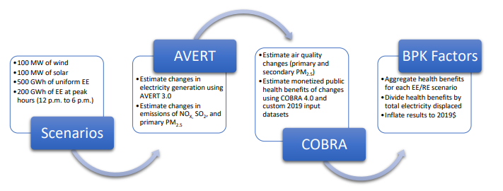 Figure 36. Overview of methods and models used in developing BPK factors
Source: U.S. EPA 2021, page 11.
This method is much simpler than using the general method described above, because the U.S. EPA has already performed many of the steps and applied the relevant models. The main disadvantage of this method is that it is limited to public health impacts of electricity generation. Estimates of public health impacts of other fuels, such as gas, oil, or gasoline, will require the general method described above.
7.2.3. Resources for Calculating Public Health Impacts
American Council for an Energy Efficient Economy. 2018. (ACEEE 2018). Cost-Effectiveness Tests: Overview of State Approaches to Account for Health and Environmental Benefits of Energy Efficiency. www.aceee.org/topic-brief/he-in-ce-testing.
American Council for an Energy Efficient Economy. 2020. (ACEEE 2020 Health). Making Health Count: Monetizing the Health Benefits of In-home services delivered by Energy Efficiency Programs. May. www.aceee.org/research-report/h2001.
Asthma and Allergy Foundation of America. 2020. (AAFA 2020). “Weather Can Trigger Asthma.” www.aafa.org/page/weather-triggers-asthma.aspx.
Burns, E., J. Stevens, and R. Lee. 2016. “The Direct Costs of Fatal and Non-Fatal Falls among Older Adults—United States.” Journal of Safety Research 58 (September): 99–103. www.sciencedirect.com/science/article/pii/S0022437516300172?via%3Dihub.
Healthcare Cost and Utilization Project. 2018. (HCUP 2018). Introduction to the HCUP National Inpatient Sample 2016. www.hcup-us.ahrq.gov/db/nation/nis/NIS_Introduction_2016.jsp.
New York City Department of Health and Mental Hygiene. 2020. (NYC DHMH 2020). “Extreme Heat and Your Health.” nyc.gov website. https://weatherization.ornl.gov/wp-content/uploads/pdf/WAPRetroEvalFinalReports/ORNL_TM-2014_345.pdf
Norton, R., B. Brown, and K. Malomo-Paris. 2017. Weatherization and Its Impact on Occupant Health Outcomes. Baltimore: GHHI (Green & Healthy Homes Initiative). www.greenandhealthyhomes.org/wp-content/uploads/Weatherization-and-its-Impact-on-Occupant-Health_Final_5_23_2017_online.pdf.
Regulatory Assistance Project. 2021. (RAP 2021). Health Benefits by the Kilowatt-Hour: Using EPA Data to Analyze the Cost-Effectiveness of Efficiency and Renewables. Nancy Seidman, John Shenot, Jim Lazar. September.
Oak Ridge National Laboratory. 2014. (ORNL 2014). Health and Household-Related Benefits Attributable to the Weatherization Assistance Program. Tonn B., E. Rose, B. Hawkins, and B. Conlon. https://weatherization.ornl.gov/wp-content/uploads/pdf/WAPRetroEvalFinalReports/ORNL_TM-2014_345.pdf
U.S. Census Bureau. 2017. “American Housing Survey (AHS) Table Creator.” census.gov website. https://www.census.gov/programs-surveys/ahs/data/interactive/ahstablecreator.html?s_areas=00000&s_year=2019&s_tablename=TABLE1&s_bygroup1=1&s_bygroup2=1&s_filtergroup1=1&s_filtergroup2=1
U.S. Centers for Disease Control and Prevention. 2019. (CDC Asthma 2019). “Asthma.” cdc.gov website. www.cdc.gov/asthma/default.htm.
U.S. Centers for Disease Control and Prevention. 2019. (CDC Hypothermia 2019). “Hypothermia.” cdc.gov website. www.cdc.gov/disasters/winter/staysafe/hypothermia.html.
U.S. Environmental Protection Agency. 2018. (U.S. EPA 2018). Quantifying the Multiple Benefits of Energy Efficiency and Renewable Energy: A Guide for State and Local Governments. www.epa.gov/statelocalenergy/quantifying-multiple-benefits-energy-efficiency-and-renewable-energy-guide-state.
U.S. Environmental Protection Agency. 2021. (U.S. EPA 2021). Public Health Benefits per kWh of Energy Efficiency and Renewable Energy in the United States: A Technical Report. www.epa.gov/statelocalenergy/public-health-benefits-kwh-energy-efficiency-and-renewable-energy-united-states.
U.S. Environmental Protection Agency. n.d. (U.S. EPA BenMAP). “Environmental Benefits Mapping and Analysis Program – Community Edition (BenMAP).” epa.gov website. www.epa.gov/benmap.
U.S. Environmental Protection Agency. n.d. (U.S. EPA COBRA). “CO-Benefits Risk Assessment Health Impacts Screening and Mapping Tool (COBRA).” epa.gov website. www.epa.gov/cobra.
U.S. Environmental Protection Agency. n.d. (U.S. EPA MOVES). “MOtor Vehicle Emission Simulator (EPA MOVES)”. epa.gov website. www.epa.gov/moves.
Wang, Srebotnjak, Brownell, and Hsia. 2014. “Emergency Department Charges for Asthma-Related Outpatient Visits by Insurance Status.” Journal of Health Care for the Poor and Underserved 25 (1): 396–405. www.muse.jhu.edu/article/536594.
7.3. Other Environmental Impacts
7.3.1. Definition
Energy resources can have a variety of environmental impacts beyond air pollutant and GHG emissions. These include environmental impacts caused by land use for generation, transmission, and distribution of energy; water consumption; solid waste disposal; liquid waste disposal; fuel mining and transportation; disposal of technologies at the end of their useful life; and more.
Most DERs will reduce these types of environmental impacts by reducing electricity, gas, and other fuel consumption. As with GHG and air emissions, some DERs might increase other environmental impacts, and some might both increase and reduce environmental impacts.
It is important to distinguish between societal environmental impacts and environmental compliance impacts (see Figure 37 and Section 3.2.6.a). Societal environmental impacts represent the emissions that occur after compliance with environmental regulations and requirements. These societal impacts are referred to as “externalities” because they are external to the monetary prices of the goods that create them. The costs of compliance with environmental requirements, on the other hand, are considered “internal” costs because they are passed on to customers in electricity prices.
Air Emissions Impacts
Utility-System Impacts
Addressed in environmental compliance costs (including current and anticipated compliance costs)
Societal impacts
Externalities not addressed in environmental compliance costs
Figure 37. Utility-system vs. societal air emissions impacts
7.3.2. Methods for Calculating Other Environmental Impacts
Because of the breadth of other environmental impacts and the complexity of the methods for estimating them, describing all these methods is beyond the scope of this report. Readers looking for guidance on these impacts should refer to the relevant resources presented below.
7.3.3. Resources for Calculating Other Environmental Impacts
Lawrence Berkeley National Laboratory. 1997. (LBNL 1997). Introduction to Environmental Externality Costs. Jonathan Koomey and Florentine Krause. https://citeseerx.ist.psu.edu/viewdoc/download?doi=10.1.1.462.503&rep=rep1&type=pdf
Oak Ridge National Laboratory. 1992. (ORNL 1992). External Costs and Benefits of Fuel Cycles. Report No. 1 of the U.S. – European Commission Fuel Cycle Study. November. inis.iaea.org/collection/NCLCollectionStore/_Public/24/047/24047135.pdf
Pace University Center for Environmental Legal Studies. 1993. (Pace 1993). Incorporation of Environmental Externalities in the United States of America. Richard Ottinger. link.springer.com/chapter/10.1007/978-3-642-76712-8_25.
Regulatory Assistance Project. 2013. (RAP 2013). Recognizing the Full Value of Energy Efficiency. J. Lazar and K. Colburn. https://www.raponline.org/wp-content/uploads/2016/05/rap-lazarcolburn-layercakepaper-2013-sept-09.pdf
U.S. Environmental Protection Agency. 2015. (U.S. EPA 2015). Benefit and Cost Analysis for the Effluent Limitations Guidelines and Standards for the Steam Electric Power Generating Point Source Category. Office of Water. September. www.epa.gov/sites/default/files/2015-10/documents/steam-electric_benefit-cost-analysis_09-29-2015.pdf.
U.S. Environmental Protection Agency. 2018. (U.S. EPA 2018). Quantifying the Multiple Benefits of Energy Efficiency and Renewable Energy: A Guide for State and Local Governments. www.epa.gov/statelocalenergy/quantifying-multiple-benefits-energy-efficiency-and-renewable-energy-guide-state.
7.4. Macroeconomic Impacts
Jurisdictions that have a policy goal of using energy investments to promote macroeconomic benefits should account for these impacts when assessing the cost-effectiveness of DERs, consistent with the guidance in the NSPM. Section 7.4.2 describes methods that can be used to estimate macroeconomic impacts for this purpose.
Avoiding double-counting macroeconomic impacts: Section 7.4.3 explains that the dollar values of macroeconomic impacts should not be simply added to the dollar values of the other impacts in the BCA, because there is too much overlap between macroeconomic impacts and utility system impacts. Instead, the macroeconomic impacts should be estimated and presented separately from the results of the BCA, to avoid double-counting of the overlapping impacts.
Note: This approach, presenting the macroeconomic results separately from the BCA results, is consistent with the approach of treating rate impacts separately from the BCA (see NSPM 2020, Appendix A) and with the approach of treating equity issues separately from the BCA results (see Chapter 9).
7.4.1. Definition
Investments in DERs will result in employment and other macroeconomic impacts. Table 71 shows the most frequently used indicators of macroeconomic development.
Table 71. Typical indicators of macroeconomic development
| Job-years |
A job-year is equivalent to a full-time employment opportunity for one person for one year (e.g., five job-years could be five jobs for one year or one job for five years). |
| Personal income |
This refers to all income collectively received by all individuals or households. Personal income includes compensation from several sources including salaries, wages, and bonuses received from employment or self-employment. |
| State GDP |
This is the total monetary or market value of all the finished goods and services produced within a state’s borders. |
| State tax revenues |
These come from property taxes, sales and gross receipts taxes, and individual income tax due to increased economic activity and employment within the state. |
These different indicators of macroeconomic development are interrelated and overlap in several ways (see Synapse 2021 RI, page 13). Therefore, these indicators should not be added together.
Macroeconomic development impacts from energy resource investments include the three categories of impacts shown in Table 72 below.
Table 72. Three categories of macroeconomic development impacts from energy resource investments
| Direct impacts |
Jobs and economic activity associated with constructing, installing, and operating the energy resource. |
| Indirect impacts |
Jobs and economic activity associated with additional work and revenue that such programs funnel to the supply chains associated with the direct impacts. These supply chains include contractors, builders/developers, equipment vendors, product retailers, distributors, manufacturers, and other elements. |
| Induced impacts |
Jobs and economic activity created by the re-spending of the newly hired workers who gained employment in the direct or indirect impacts categories. |
Investments in energy resource can have both positive and negative macroeconomic impacts. First, there is the positive impact caused by installing, operating, and maintaining the energy resource. Second, there may be a negative macroeconomic effect caused by avoiding or displacing other energy resources.
In addition, when customers experience a reduction in their utility bills, this money saved is assumed to be put back into the economy somehow, leading to additional macroeconomic development. This is referred to as the customer “respending” effect. When utility investments reduce utility bills on average, the customer respending effect leads to increased macroeconomic development. When utility investments increase utility bills on average, the customer respending effect leads to decreased macroeconomic development.
DERs create macroeconomic impacts in two different phases. The first phase is during the installation of the DER, which might last as long as a year or two. The second phase is during the operation of the DER, which lasts many years. In the second phase, most of the job and economic activity impacts are created from the reductions or increases in energy costs which lead to customer respending effects (see ACEEE 2019, page 2).
7.4.2. Methods for Calculating Macroeconomic Development Impacts
Table 73 describes approaches for estimating macroeconomic development impacts. For each method, macroeconomic development impacts are estimated by comparing the economic outcomes under the Reference Case to the economic outcomes associated with the DER Case. The difference between the two cases is the net macroeconomic impact attributable to the DERs.
Table 73. Macroeconomic development impacts: methods and models
| Method |
Description |
Typical Use |
| Rules-of-thumb factors |
Generic rules-of-thumb factors are simplified factors that represent relationships between key policy or program characteristics (e.g., financial spending, energy savings) and employment or output. |
High-level screening analysis |
| Input-output models |
Input-output models, also known as multiplier analysis models, can also be used to conduct analyses within a limited budget and timeframe, but provide more rigorous results than those derived from rules of thumb. |
Short-term analysis of investments with limited scope and impact |
| Econometric models |
Econometric models use mathematical and statistical techniques to analyze economic conditions both in the present and in the future to forecast how investments might affect income, employment, gross state product, and other common output metrics. |
Short- and long-term analysis of investments with an economy-wide impact |
| Computable general equilibrium models (CGE) |
CGE models use equations derived from economic theory to trace the flow of goods and services throughout an economy and solve for the levels of supply, demand, and prices across a specified set of markets. |
Long-term analysis of Investments with an economy-wide impact |
| Hybrid models |
Hybrid models typically combine aspects of CGE modeling with those of econometric models and may be based more heavily on one or the other. |
Short- and long-term analysis of investments with a limited or economy-wide impact |
Notes: Adapted from U.S. EPA 2018, Part 2, Chapter 5, Table 5-1. See this reference for a detailed discussion of the strengths and limitations of each approach.
Input-output modeling is one of the most frequently used methods to estimate macroeconomic development impacts given its relatively low cost and flexibility. Two common input-output models used to estimate the macroeconomic development impacts are:
- REMI (Regional Economic Models Inc.) Model. REMI is a proprietary dynamic forecasting and policy analysis tool. The model forecasts the future of a regional economy, and it predicts the effects on that same economy when the user implements a change. REMI models have been used throughout the world for a wide range of topic areas, including macroeconomic development, the environment, energy, transportation, and taxation, forecasting, and planning.
- IMPLAN (Economic Impact Analysis for Planning, IMPLAN Group, LLC). IMPLAN is a propriety, industry-standard input-output model that accounts for both the direct and indirect economic impact of an industry. IMPLAN was developed by the U.S. Forest Service in the 1970s to deliver accurate and timely estimates of economic impacts of forest resources.
These models are very comprehensive and address many aspects of the economy being modeled. Consequently, they require users to make assumptions and decisions in order to process the model outputs. For example, users often need to make assumptions about the flow of money within and outside of a state in order to determine in-state impacts.
It is important to set the appropriate boundary for the macroeconomic analysis. Macroeconomic development impacts from DERs can occur within a state, neighboring states, the entire United States, and even other countries. Most jurisdictions are interested in the macroeconomic development impacts within the state where the DER is implemented. In such cases, the in-state macroeconomic impacts should be isolated from the rest of the impacts.
Macroeconomic impacts should include increased macroeconomic development from increased utility and customer spending, plus reduced macroeconomic development from reduced utility spending, plus the customer respending effect.
Note that utility spending can lead to both an increase and a decrease in macroeconomic development. In the case of DERs, the increased development is the result of the purchase, installation, and maintenance of DERs, while the decreased macroeconomic development results from investments in generation, transmission, and distribution facilities that were avoided by the DERs. The macroeconomic impact of any energy resource should include the net macroeconomic effects, (i.e., both the increases and the decreases in macroeconomic development).
In sum, macroeconomic impacts should include increased macroeconomic development from increased utility and customer spending, plus reduced macroeconomic development from reduced utility spending, plus the customer respending effect.
Table 74 presents a summary of the methods for estimating macroeconomic impacts, including advantages and disadvantages of each method.
Table 74. Summary of methods for estimating macroeconomic impacts of energy resources
| Tool |
Description |
Application |
Advantages |
Disadvantages |
| Adders and multipliers |
A simple factor to scale up resource benefits to include or estimate economic development benefits from a given resource benefit amount |
Once adder is determined or multiplier is estimated, can be applied to resource benefits estimates using simple arithmetic |
Simplicity, transparency, ease of use, relatively low cost (adders more so than multipliers) |
Limited accuracy, adders sometimes set somewhat arbitrarily |
| Input-output models |
A relatively simple model that calculates benefits based on number of jobs required to sustain a given economic activity or the GDP created by economic activity |
Practitioners must input the level of resources being invested and the savings they generate as well as the investment costs and other key parameters |
Less expensive and easier to use than other types of models; transparent |
Limited ability to assess impact of price changes; often do not assess changes over time |
| Econometric models |
A more complicated model that relates changes in individual sectors and prices to one another and the economy as a whole |
Typically require experienced modelers to program the investments and other key parameters |
Thoroughly represent interactions between sectors and changes over time |
Expensive; results heavily influenced by opaque parameters estimated by the modeler |
| CGE and hybrid models |
A typically less-detailed model of the economy with relationships governed by economic theory and estimated parameters |
Typically require experienced modelers to program investments and other key parameters |
Theoretically consistent results; can project long-term impacts; available at state and local levels; hybrid models allow for unexploited investment opportunities |
Expensive; results heavily influenced by opaque parameters and assumptions; unavailable at subnational levels; traditional CGE models assume a state of economic equilibrium |
Source: Adapted from ACEEE 2019, page 8.
7.4.3. Role of Macroeconomic Development Impacts in a BCA
Consistent with NSPM guidance, monetary estimates of macroeconomic development impacts should not be added to the monetary cost-effectiveness analysis results, because they represent a different type of economic impact. The macroeconomic development benefits represent economic activity in the state, which is different from the customer and societal impacts included in an energy efficiency program BCA. Further, there are several aspects of BCAs and macroeconomic development analyses that overlap; therefore, adding the macroeconomic development results directly onto the BCA results will result in double-counting some of the effects (see NSPM 2020; Synapse 2019, Appendix B).
Figure 38 presents a comparison of the key elements of BCAs and macroeconomic development analyses. It indicates how some elements (e.g., benefits and costs) of a BCA may overlap with elements of the macroeconomic development analysis, resulting in significant overlap:
- The utility system benefits, in terms of avoided costs, result in reduced spending that leads to reduced economic activity.
- The utility system costs, in terms of resource investments, result in increased spending that leads to increased economic activity.
- The customer bill impacts, which are the difference between the utility system benefits and costs, result in customer respending effects that also lead to economic activity. Note that the customer bill impacts are not an additional cost or benefit in the BCA. Instead, they are an output of the BCA, equal to the utility system benefits minus the utility system costs. The bill impacts are separated out in the BCA portion of this graphic to make the point that those impacts are what lead to the customer respending effect in the macroeconomic impact analyses.
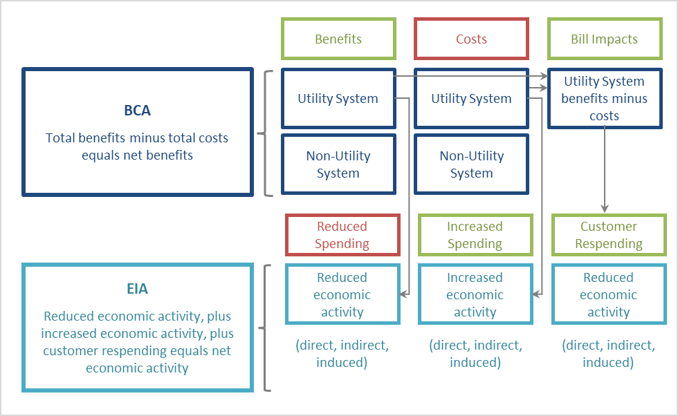 Figure 38. Comparison of benefit-cost analyses and macroeconomic impact analyses (EIA)
Source: Synapse 2021 RI.
Another way to describe the overlap between benefits and costs of DER BCAs and macroeconomic development analyses is that the cost of the goods and services purchased (or not purchased) as a result of the utility investment are included in the BCA, and they are also included in the macroeconomic development analyses in terms of the direct and indirect economic activity. There is not, however, a one-to-one relationship between the BCA impacts and the macroeconomic development impacts. In other words, a dollar spent on a utility investment in the BCA is not equivalent to a dollar of economic activity (GDP or otherwise) in the macroeconomic development analysis. This makes it very difficult, if not impossible, to separate the macroeconomic development impacts from the other BCA impacts.
Further, BCAs and macroeconomic development analyses serve two different purposes. BCAs are intended to indicate the costs and benefits to utilities, customers, and society (depending upon the perspective chosen), while macroeconomic development analyses are intended to show distributional impacts across different parties within society (see U.S. EPA, pages 11-2 through 11-9). Therefore, combining dollar values of one analysis with another would conflate the purposes and the findings of both of them.
While the macroeconomic development impacts should not be added directly to the dollar values in the BCA, they can nonetheless be accounted for in the decision-making process. This can be achieved by presenting the macroeconomic development impacts alongside the monetary results of the BCA (see U.S. EPA 2014, page 11-2). This approach allows utilities, stakeholders, and regulators the opportunity to review and understand the macroeconomic development impacts of the DER Case, and to use those impacts in informing the ultimate decision on whether the DERs are cost-effective.
While the macroeconomic development impacts should not be added directly to the dollar values in the BCA, they can nonetheless be accounted for in the decision-making process. This can be achieved by presenting the macroeconomic development impacts alongside the monetary results of the BCA.
The number of net job-years is the most useful metric to present alongside BCA results, because job growth is easily understood by a wide variety of stakeholders. The other indicators, such as net changes in GDP, personal income, and state tax revenues, can also be used as long as an explanation is provided about what each represents.
7.4.4. Resources for Calculating Macroeconomic Development Impacts
American Council for an Energy Efficient Economy. 2019. (ACEEE 2019). State Policy Toolkit: Guidance on Measuring the Economic Development Benefits of Energy Efficiency. www.aceee.org/sites/default/files/Jobs%20Toolkit%203-8-19.pdf.
Brattle Group. 2019. Review of RI Test and Proposed Methodology, prepared for National Grid.
Synapse Energy Economics. 2021. (Synapse 2021 RI). Macroeconomic Impacts of the Rhode Island Community Remote Net Metering Program. Prepared for the Rhode Island Division of Public Utilities and Carriers. March. www.ripuc.ri.gov/generalinfo/Synapse-CRNM-Macroeconomic-Report-2021.pdf.
U.S. Environmental Protection Agency. Updated 2014. (U.S. EPA 2014). Guidelines for Preparing Economic Analyses. National Center for Environmental Economics, Office of Policy. www.epa.gov/sites/default/files/2017-08/documents/ee-0568-50.pdf.
U.S. Environmental Protection Agency. 2018. (U.S. EPA 2018). Quantifying the Multiple Benefits of Energy Efficiency and Renewable Energy: A Guide for State and Local Governments. www.epa.gov/statelocalenergy/quantifying-multiple-benefits-energy-efficiency-and-renewable-energy-guide-state.
7.5. Energy Security
Beyond the societal impacts discussed above, some jurisdictions may have policy goals supporting investment in DERs related to increasing energy security in the form of cybersecurity and/or energy independence. These impacts are described below; however, there is limited guidance on types of methods for quantifying these impacts. Further research on, and development of, methodological approaches is warranted to assist jurisdictions in being able to account for these impacts in assessing DER investments—the value of which is not zero, in particular with regard to cybersecurity given critical concerns in this area.
7.5.1. Definition
Cybersecurity is one aspect of energy security that DERs might affect. Many DERs are networked (i.e., connected to the internet or considered “smart” devices). Such DERs can include electric vehicles, electric vehicle charging stations, smart inverters, and devices with smart meters. These types of devices connected to the grid’s distribution system potentially introduce cybersecurity vulnerabilities. Not only do potential cyberattacks and surveillance issues present a risk to the owner of the devices, but they also present a risk to the distribution grid.
As the prevalence of DERs increases, they may make distribution systems more vulnerable to cybersecurity attacks (see GAO 2021, NREL 2019). For example, attackers may be able to compromise a large number of high-wattage networked DERs (e.g., smart water heaters) and use them in a coordinated attack to disrupt grid operations. Best practices and standards for preventing DER-related cyberattacks are still being developed by North American Electric Reliability Corporation and National Institute of Standards and Technology (see NREL 2019).
Energy independence is another aspect of energy security that DERs might affect. DER investments that reduce energy imports from outside the jurisdiction, state, region, or country can help advance the goals of energy independence and security. The following quote describes the relationship between distributed resources and energy security:
Energy independence can improve energy security, for example when using domestic energy efficiency and renewable energy resources to reduce dependence on foreign fuel sources. Avoiding the use of imported petroleum may yield political and economic benefits by protecting consumers from supply shortages and price shocks. Energy and national security are also improved when the existence of one easily targeted large unit with onsite fuel is replaced with many smaller units that are located in a variety of locations. (See U.S. EPA 2018, page 3-40.)
Several DERs—including electric vehicles, heat pumps, distributed solar PV, energy storage, and to some extent energy efficiency—reduce reliance on fossil fuels in the form of gasoline and diesel for internal combustion engine vehicles; natural gas, propane, or oil for home heating end-uses; and oil, coal, or natural gas for supplying electricity to the grid. Therefore, some DERs can improve energy security by reducing the amount of petroleum imported into the jurisdiction where the DER is located.
7.5.2. Methods for Accounting for Energy Security Impacts
7.5.2.a. Cybersecurity
Though costs from cyberattacks are well documented, few studies, if any, include the potential costs of cyberattacks in their cost-effectiveness tests for DERs.20 This may be due to several factors, including:
- The low penetration of networked DERs to date;
- The uncertainty of the magnitude of potential DER-related cyberattacks; and
- The development of IEEE 1547.3 cybersecurity standards and protocols of networked DERs as their proliferation increases.
7.5.2.b. Energy Independence
Thus far, no studies known to the authors have attempted to estimate the value to energy independence from DER adoption. According to the U.S. EPA, energy security is a benefit of energy efficiency and renewable energy that has associated cost reductions, but the methodologies for quantifying them are purely qualitative or subject to debate (see U.S. EPA 2018).
7.5.3. Resources for Energy Security Impacts
Government Accountability Office. 2021. (GAO 2021). Electricity Grid Cybersecurity: DOE Needs to Ensure Its Plans Fully Address Risks to Distribution Systems. March. www.gao.gov/products/gao-21-81.
Institute of Electrical and Electronics Engineers Standards Association. 2020. (IEEE SA 2020). Guide for Cybersecurity of Distributed Energy Resources Interconnected with Electric Power Systems. www.standards.ieee.org/project/1547_3.html
National Renewable Energy Laboratory. 2019. (NREL 2019). An Overview of Distributed Energy Resource (DER) Interconnection: Current Practices and Emerging Solutions. April. www.nrel.gov/docs/fy19osti/72102.pdf.
Radware. 2019. 2018-2019 Global Application & Network Security Report. www.radware.com/ert-report-2018/.
U.S. Environmental Protection Agency. 2018. (U.S. EPA 2018). Quantifying the Multiple Benefits of Energy Efficiency and Renewable Energy: A Guide for State and Local Governments. www.epa.gov/statelocalenergy/quantifying-multiple-benefits-energy-efficiency-and-renewable-energy-guide-state.
16 Methods for calculating refrigerant leaks are not addressed in this handbook. For guidance on how to estimate refrigerant leaks, see CA ACC 2020, pages 79-81.
17 Note that upstream leakage rates should represent marginal, not average, leakage rates because DERs will affect marginal leakages.
18 One of the more obvious factors affecting the magnitude of the SCC is the discount rate. For example, the SCC for 2020 is estimated to be either 49, 116, or 390 $/ton, depending upon whether a discount rate of 3%, 2%, or 1% is used, respectively (AESC 2021, page 179). However, there are many other, less obvious, assumptions that have significant implications for the magnitude of the SCC, including the choice of models used, the inputs to those models, and the interpretation of the model results (Ackerman 2008).
19 There have already been public health impacts of climate change to date, due to the severe weather events exacerbated by climate change. Nonetheless, the theory behind the marginal abatement cost approach is that if the societal goal of reducing GHG emissions is achieved, the vast majority of future climate change impacts, including public health impacts, can be prevented.
20 According to Radware, the cost of a cyberattack in 2018 and 2019 was about $1.1 million (see Radware 2019).